As the title reads, in this heterogeneous session we will see three topics of different interest. The first is a collection of three simple and useful one-function R packages that I use regularly in my coding workflow. The second collects some approaches to handling and performing linear regression with big data. The third brings in the freaky component: it presents tools to display graphical information in plain ASCII, from bivariate contours to messages from Yoda!
You can download the script with the R code alone here (right click and “Save as…”).
We will need the following packages:
install.packages(c("viridis", "microbenchmark", "multcomp", "manipulate",
                   "ffbase", "biglm", "leaps", "txtplot", "NostalgiR",
                   "cowsay"),
                 dependencies = TRUE)
Some simple and useful R packages
Color palettes with viridis
Built-in color palettes in base R are somehow limited. We have rainbow, topo.colors, terrain.colors, heat.colors, and cm.colors. We also have flexibility to create our own palettes, e.g. by using colorRamp. These palettes look like:
# MATLAB's color palette
jet.colors <- colorRampPalette(c("#00007F", "blue", "#007FFF", "cyan",
                                 "#7FFF7F", "yellow", "#FF7F00", "red",
                                 "#7F0000"))
# Plot for palettes
testPalette <- function(col, n = 200, ...) {
  image(1:n, 1, as.matrix(1:n), col = get(col)(n = n, ...),
        main = col, xlab = "", ylab = "", axes = FALSE)
}

# Color palettes comparison
par(mfrow = c(2, 3))
res <- sapply(c("rainbow", "topo.colors", "terrain.colors",
                "heat.colors", "cm.colors", "jet.colors"), testPalette)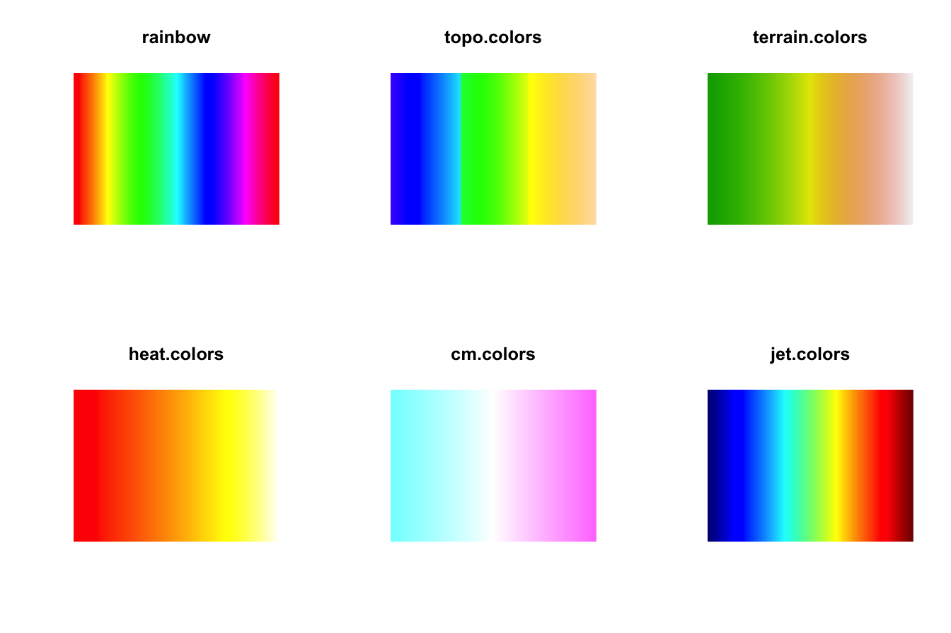
Notice that some palettes clearly show non-uniformity in the color gradient. This potentially leads to an interpretation bias when inspecting heatmaps colored by these scales: some features are (unfairly) weakened and others are (unfairly) strengthen. This distortion on the representation of the data can be quite misleading.
In addition to these problems, some problematic points that are not usually thought when choosing a color scale are:
- How does your pretty color image look like when you print it in black-and-white?
- How do colorblind people read the images?
The package viridisLite (a port from Python’s Matplotlib) comes to solve these three issues. It provides the viridis color palette, which uses notions from color theory to be as much uniform as possible, black-and-white-ready, and colorblind-friendly. From viridisLite’s help:
This color map is designed in such a way that it will analytically be perfectly perceptually-uniform, both in regular form and also when converted to black-and-white. It is also designed to be perceived by readers with the most common form of color blindness.
More details can be found in this great talk by one of the authors:
There are several palettes in the package. All of them have the same properties as viridis (i.e., perceptually-uniform, black-and-white-ready, and colorblind-friendly). The cividis is specifically aimed to people with color vision deficiency. Let’s see them in action:
library(viridisLite)
# Color palettes comparison
par(mfrow = c(2, 3))
res <- sapply(c("viridis", "magma", "inferno", "plasma", "cividis"),
              testPalette)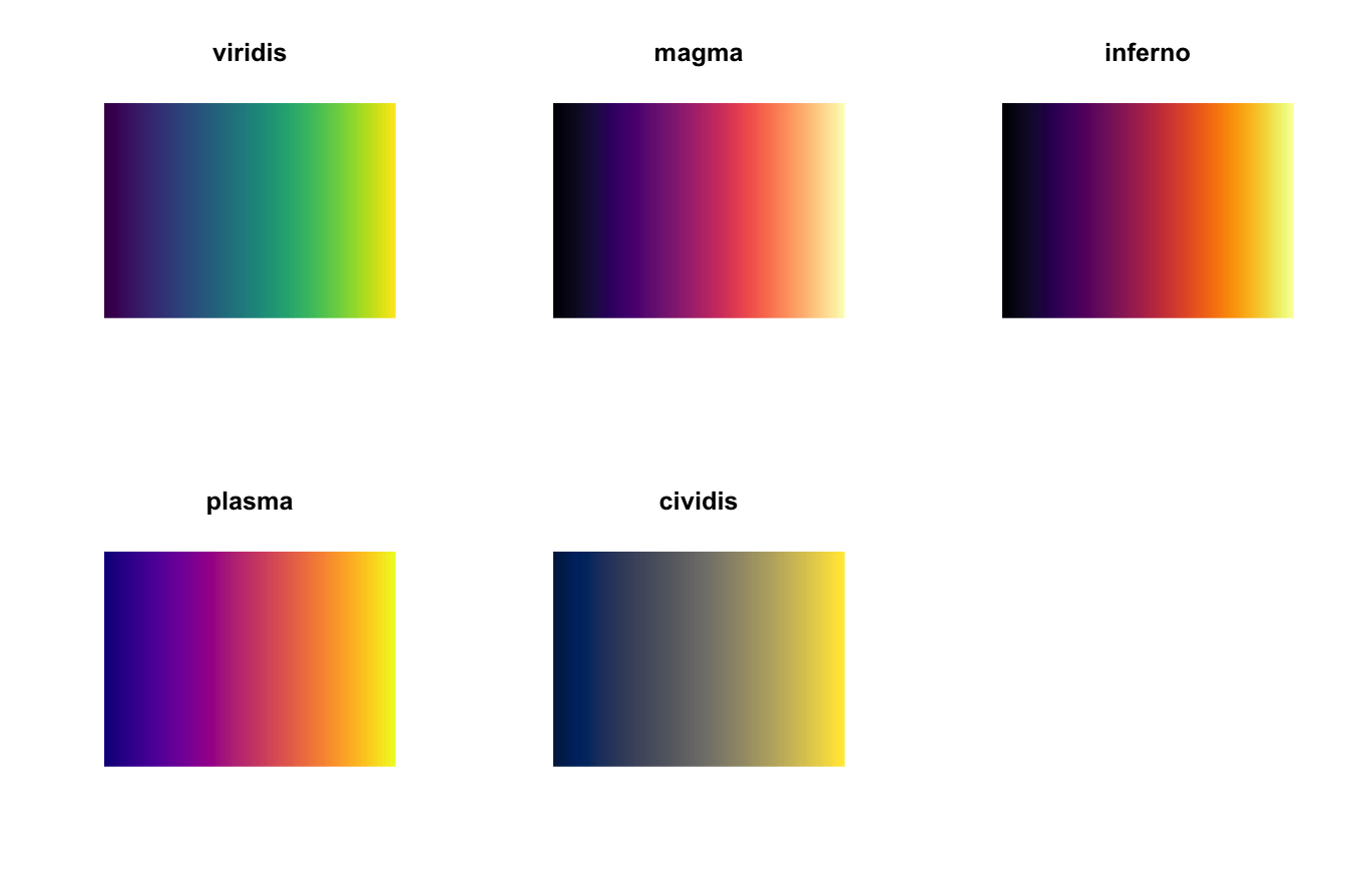
Some useful options for any of the palettes are:
# Reverse palette
par(mfrow = c(1, 2))
testPalette("viridis", direction = 1)
testPalette("viridis", direction = -1)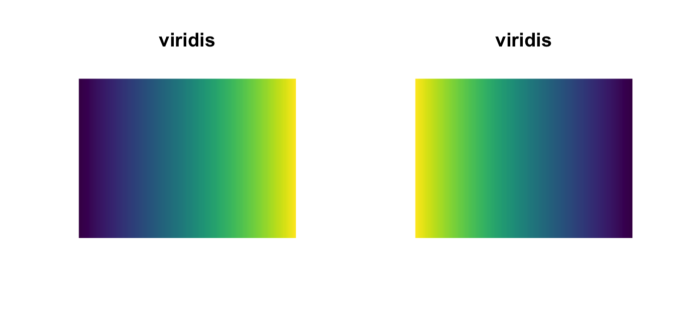
# Truncate color range
par(mfrow = c(1, 2))
testPalette("viridis", begin = 0, end = 1)
testPalette("viridis", begin = 0.25, end = 0.75)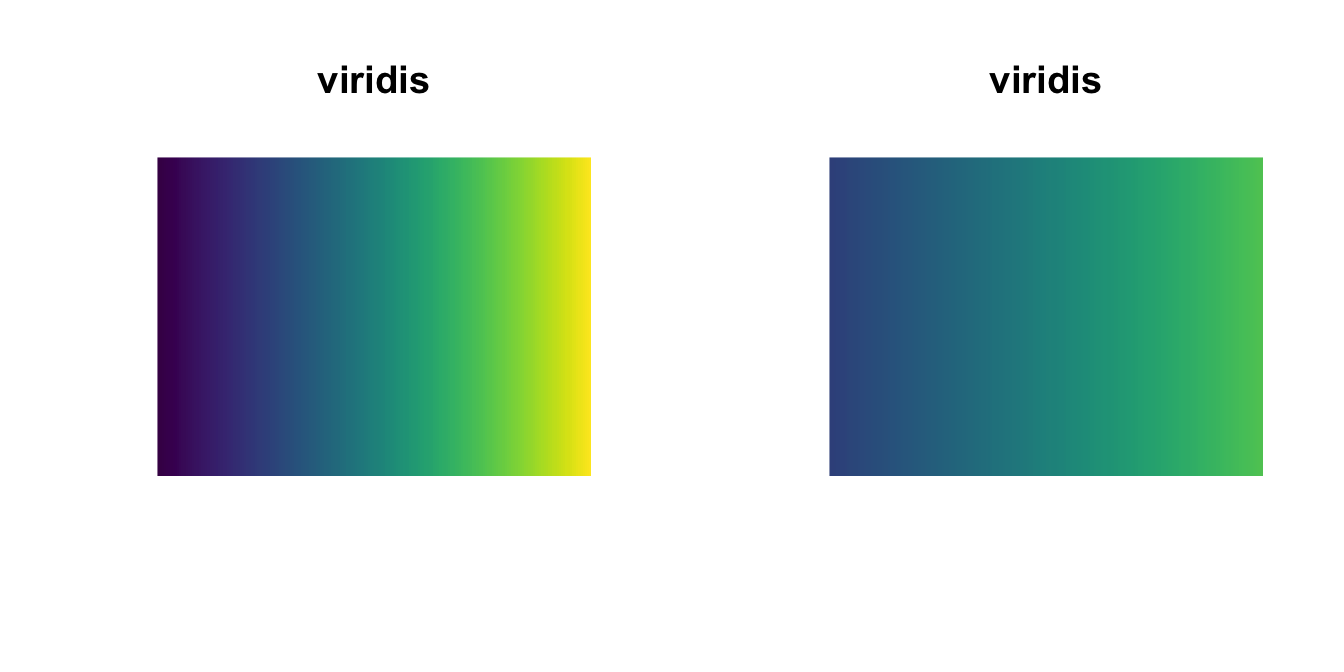
# Asjust transparency
par(mfrow = c(1, 2))
testPalette("viridis", alpha = 1)
testPalette("viridis", alpha = 0.5)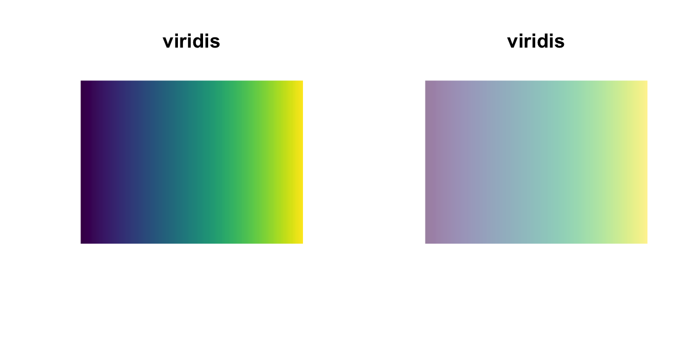
In the extended viridis package there are color palettes functions for ggplot2 fans: scale_color_viridis and scale_fill_viridis. Some examples of their use:
library(viridis)
library(ggplot2)

# Using scale_color_viridis
ggplot(mtcars, aes(wt, mpg)) +
  geom_point(size = 4, aes(color = factor(cyl))) +
  scale_color_viridis(discrete = TRUE) +
  theme_bw()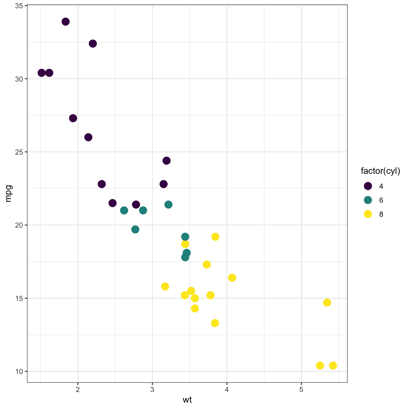
# Using scale_fill_viridis
dat <- data.frame(x = rnorm(1e4), y = rnorm(1e4))
ggplot(dat, aes(x = x, y = y)) +
  geom_hex() + coord_fixed() +
  scale_fill_viridis() + theme_bw()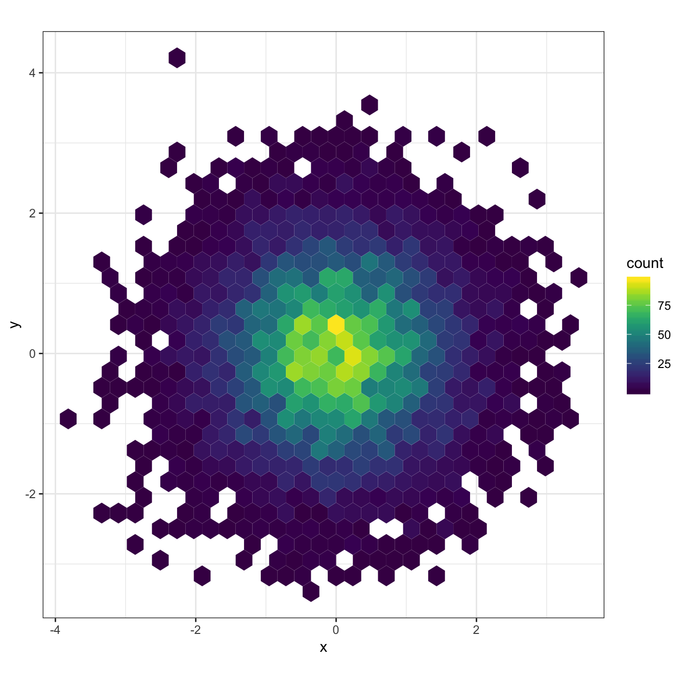
Benchmarking with microbenchmark
Measuring the code performance is a day-to-day routine for many developers. It is also a requirement for regular users that want to choose the most efficient coding strategy for implementing a method.
As we know, we can measure running times in base R using proc.time or system.time:
# Using proc.time
time <- proc.time()
for (i in 1:100) rnorm(100)
time <- proc.time() - time
time # elapsed is the 'real' elapsed time since the process was started
## user system elapsed
## 0.003 0.000 0.003# Using system.time - a wrapper for the above code
system.time({for (i in 1:100) rnorm(100)})## user system elapsed
## 0.002 0.000 0.003However, this very basic approach presents several inconveniences to be aware of:
- The precision of
proc.timeis within the millisecond. This means that evaluating1:1000000(usually) takes0seconds at the sight ofproc.time. - Each time measurement of a procedure is subjected to variability (depends on the processor usage at that time, processor warm-up, memory status, etc). So, one single call is not enough to assess the time performance, several must be made (conveniently) and averaged.
- It is cumbersome to check the times for different expressions. We will need several lines of code for each and creating auxiliary variables.
- There is no summary of the timings. We have to code it by ourselves.
- There is no checking on the equality of the results outputted from different approaches (accuracy is also important, not only speed!). Again, we have to code it by ourselves.
Hopefully, the microbenchmark package fills in these gaps. Let’s see an example of its usage on approaching a common problem in R: how to recentre a matrix by columns, i.e., how to make each column to have zero mean. There are several possibilities to do so, with different efficiencies.
# Data and mean
n <- 3
m <- 10
X <- matrix(1:(n * m), nrow = n, ncol = m)
mu <- colMeans(X)
# We assume mu is given in the time comparisons
Time to think by yourself on the competing approaches! Do not cheat and do not look into the next chunk of code!
# SPOILER ALERT!
#
#
#
#
#
#
#
#
#
#
#
#
#

# Some approaches:

# 1) sweep
Y1 <- sweep(x = X, MARGIN = 2, STATS = mu, FUN = "-")

# 2) apply (+ transpose to maintain the arrangement of X)
Y2 <- t(apply(X, 1, function(x) x - mu))

# 3) scale
Y3 <- scale(X, center = mu, scale = FALSE)

# 4) loop
Y4 <- matrix(0, nrow = n, ncol = m)
for (j in 1:m) Y4[, j] <- X[, j] - mu[j]

# 5) magic (my favourite!)
Y5 <- t(t(X) - mu)
Which one do you think is faster? Do not cheat and answer before seeing the output of the next chunk of code!
# Test speed
library(microbenchmark)
bench <- microbenchmark(
  sweep(x = X, MARGIN = 2, STATS = mu, FUN = "-"),
  t(apply(X, 1, function(x) x - mu)),
  scale(X, center = mu, scale = FALSE),
  {for (j in 1:m) Y4[, j] <- X[, j] - mu[j]; Y4},
  t(t(X) - mu)
)

# Printing a microbenchmark object gives a numerical summary
bench
# Notice the last column. It is only present if the package multcomp is present.
# It provides a statistical ranking (accounts for which method is significantly
# slower or faster) using multcomp::cld

# Adjusting display
print(bench, unit = "ms", signif = 2)
# unit = "ns" (nanosecs), "us" ("microsecs"), "ms" (millisecs), "s" (secs)

# Graphical methods for the microbenchmark object
# Raw time data
par(mfrow = c(1, 1))
plot(bench, names = c("sweep", "apply", "scale", "for", "recycling"))
# Employs time logarithms
boxplot(bench, names = c("sweep", "apply", "scale", "for", "recycling"))
# Violin plots
autoplot(bench)

# microbenchmark uses 100 evaluations and 2 warmup evaluations (these are not
# measured) by default. Here is how to change these dafaults:
bench2 <- microbenchmark(
  sweep(x = X, MARGIN = 2, STATS = mu, FUN = "-"),
  t(apply(X, 1, function(x) x - mu)),
  scale(X, center = mu, scale = FALSE),
  {for (j in 1:m) Y4[, j] <- X[, j] - mu[j]; Y4},
  t(t(X) - mu),
  times = 1000, control = list(warmup = 10)
)
bench2

# Let's check the accuracy of the methods as well as their timings. For that
# we need to define a check function that takes as input a LIST with each slot
# representing the output of each method. The check must return TRUE or FALSE
check1 <- function (results) {
  all(sapply(results[-1], function(x) {
    max(abs(x - results[[1]]))
    }) < 1e-15) # Compares all results pair-wisely with the first
}

# Example with check function
bench3 <- microbenchmark(
  sweep(x = X, MARGIN = 2, STATS = mu, FUN = "-"),
  t(apply(X, 1, function(x) x - mu)),
  scale(X, center = mu, scale = FALSE),
  {for (j in 1:m) Y4[, j] <- X[, j] - mu[j]; Y4},
  t(t(X) - mu),
  check = check1
)
bench3
Quick animations with manipulate
The manipulate package (works only within RStudio!) allows to easily create simple animations. It is a simpler, local, alternative to Shiny applications.
library(manipulate)

# A simple example
manipulate({
  plot(1:n, sin(2 * pi * (1:n) / 100), xlim = c(1, 100), ylim = c(-1, 1),
       type = "o", xlab = "x", ylab = "y")
  lines(1:100, sin(2 * pi * 1:100 / 100), col = 2)
}, n = slider(min = 1, max = 100, step = 1, ticks = TRUE))
# Illustrating several types of controls using the kernel density estimator
manipulate({
# Sample data
if (newSample) {
set.seed(sample(1:1000))
} else {
set.seed(12345678)
}
samp <- rnorm(n = n, mean = 0, sd = 1.5)
# Density estimate
plot(density(x = samp, bw = h, kernel = kernel),
xlim = c(-x.rang, x.rang)/2, ylim = c(0, y.max))
# Show data
if (rugSamp) {
rug(samp)
}
# Add reference density
if (realDensity) {
tt <- seq(-x.rang/2, x.rang/2, l = 200)
lines(tt, dnorm(x = tt, mean = 0, sd = 1.5), col = 2)
}
},
n = slider(min = 1, max = 250, step = 5, initial = 10),
h = slider(0.05, 2, initial = 0.5, step = 0.05),
x.rang = slider(1, 10, initial = 6, step = 0.5),
y.max = slider(0.1, 2, initial = 0.5, step = 0.1),
kernel = picker("gaussian", "epanechnikov", "rectangular",
"triangular", "biweight", "cosine", "optcosine"),
rugSamp = checkbox(TRUE, "Show rug"),
realDensity = checkbox(TRUE, "Draw real density"),
newSample = button("New sample!")
)# Another example: rotating 3D graphs without using rgl
# Mexican hat
x <- seq(-10, 10, l = 50)
y <- x
f <- function(x, y) {r <- sqrt(x^2 + y^2); 10 * sin(r)/r}
z <- outer(x, y, f)
# Colors
nrz <- nrow(z)
ncz <- ncol(z)
zfacet <- z[-1, -1] + z[-1, -ncz] + z[-nrz, -1] + z[-nrz, -ncz]
col <- viridis(100)
facetcol <- cut(zfacet, length(col))
col <- col[facetcol]
# 3D plot
manipulate(
persp(x, y, z, theta = theta, phi = phi, expand = 0.5, col = col,
ticktype = "detailed", xlab = "X", ylab = "Y", zlab = "Sinc(r)"),
theta = slider(-180, 180, initial = 30, step = 5),
phi = slider(-90, 90, initial = 30, step = 5))Handling big data in R
The ff and ffbase packages
R stores all the data in RAM, which is where all the processing takes place. But when the data does not fit into RAM (e.g., vectors of size \(2\times 10^9\)), alternatives are needed. ff is an R package for working with data that does not fit in RAM. From ff’s description:
The
ffpackage provides data structures that are stored on disk but behave (almost) as if they were in RAM by transparently mapping only a section (pagesize) in main memory - the effective virtual memory consumption perffobject.
The package ff lacks some standard statistical methods for operating with ff objects. These are provided by ffbase.
Let’s see an example.
# Not really "big data", but for the sake of illustration
set.seed(12345)
n <- 1e6
p <- 10
beta <- seq(-1, 1, length.out = p)^5

# Data for linear regression
x1 <- matrix(rnorm(n * p), nrow = n, ncol = p)
x1[, p] <- 2 * x1[, 1] + rnorm(n, sd = 0.1)
x1[, p - 1] <- 2 - x1[, 2] + rnorm(n, sd = 0.5)
y1 <- 1 + x1 %*% beta + rnorm(n)
bigData1 <- data.frame("resp" = y1, "pred" = x1)

# Data for logistic regression
x2 <- matrix(rnorm(n * p), nrow = n, ncol = p)
y2 <- rbinom(n = n, size = 1, prob = 1 / (1 + exp(-(1 + x2 %*% beta))))
bigData2 <- data.frame("resp" = y2, "pred" = x2)

# Sizes of objects
print(object.size(bigData1), units = "Mb")
print(object.size(bigData2), units = "Mb")

# Save files to disk to emulate the situation with big data
write.csv(x = bigData1, file = "bigData1.csv", row.names = FALSE)
write.csv(x = bigData2, file = "bigData2.csv", row.names = FALSE)

# Read files using ff
library(ffbase) # Imports ff
bigData1ff <- read.table.ffdf(file = "bigData1.csv", header = TRUE, sep = ",")
bigData2ff <- read.table.ffdf(file = "bigData2.csv", header = TRUE, sep = ",")

# Recall: the *.csv are not copied into RAM!
print(object.size(bigData1ff), units = "Kb")
print(object.size(bigData2ff), units = "Kb")

# Delete the csv files in disk
file.remove(c("bigData1.csv", "bigData2.csv"))
Operations on ff objects are carried out similarly as with regular data.frames:
# Operations on ff objects "almost" as with regular data.frames
class(bigData1ff)
class(bigData1ff[, 1])
bigData1ff[1:5, 1] <- rnorm(5)
# See ?ffdf for more allowed operations

# Filter of data frames
ffwhich(bigData1ff, bigData1ff$resp > 5)
Regression using biglm and friends
The richness of information returned by R’s lm has immediate drawbacks when working with big data (large \(n\), \(n>p\)). An example is the following. If \(n=10^8\) and \(p=10\), simply storing the response and the predictors takes up to \(8.2\) Gb in RAM. This is in the edge of feasibility for many regular laptops. However, calling lm will consume, at the very least, \(16.5\) Gb merely storing the residuals, effects, fitted.values, and qr decomposition. Although there are more efficient ways of performing linear regression in base R (e.g., with .lm.fit), we still need to rethink the least squares estimates computation (takes \(\mathcal{O}(np+p^2)\) in memory) to do not overflow the RAM.
A handy solution is given by the biglm package, which allows to fit a generalized linear model (glm) in R consuming much less RAM. Essentially, we have two possible approaches for fitting a glm:
Use a regular
data.frameobject to store the data, then usebiglmto fit the model. This assumes that:- We are able to store the dataset in RAM or, alternatively, that we can split it into chunks that are fed into the model iteratively, updating the fit via
udpatefor each new data chunk. - The updating must rely only in the new chunk of data, not in the full dataset (otherwise, there is no point in chunking the data). This is possible with linear models, but not possible (at least exaclty) for generalized linear models.
- We are able to store the dataset in RAM or, alternatively, that we can split it into chunks that are fed into the model iteratively, updating the fit via
Use a
ffdfobject to store the data, then useffbase’sbigglm.ffdfto fit the model.
We will focus on the second approach due to its simplicity. For an example of the use of the first approach with a linear model, see here.
Let’s see first an example of linear regression.
library(biglm)
# bigglm.ffdf has a very similar syntax to glm - but the formula interface does
# not work always as expected:
# bigglm.ffdf(formula = resp ~ ., data = bigData1ff) # Does not work
# bigglm.ffdf(formula = resp ~ pred.1 + pred.2, data = bigData1ff) # Does work,
# but not very convenient for a large number of predictors

# Hack for automatic inclusion of all the predictors
f <- formula(paste("resp ~", paste(names(bigData1ff)[-1], collapse = " + ")))

# bigglm.ffdf's call
biglmMod <- bigglm.ffdf(formula = f, data = bigData1ff, family = gaussian())
class(biglmMod)

# lm's call
lmMod <- lm(formula = resp ~ ., data = bigData1)

# The reduction in size of the resulting object is more than notable
print(object.size(biglmMod), units = "Kb")
print(object.size(lmMod), units = "Mb")

# Summaries
s1 <- summary(biglmMod)
s2 <- summary(lmMod)
s1
s2
# The summary of a biglm object yields slightly different significances for the
# coefficients than for lm. The reason is that biglm employs N(0, 1)
# approximations for the distributions of the t-tests instead of the exact
# t distribution. Obviously, if n is large, the differences are inappreciable.

# Extract coefficients
coef(biglmMod)

# AIC
AIC(biglmMod, k = 2)

# Prediction works "as usual"
predict(biglmMod, newdata = bigData1[1:5, ])
# newdata must contain a column for the response!
# predict(biglmMod, newdata = bigData2[1:5, -1]) # Error

# Update the model with more training data - this is key for chunking the data
update(biglmMod, moredata = bigData1[1:100, ])
Model selection of biglm models can be done with the leaps package. This is achieved by the regsubsets function, which returns the best subset of up to (by default) nvmax = 8 predictors. The function requires the full biglm model to begin the “exhaustive” search, in which is crucial the linear structure of the estimator.
# Model selection adapted to big data models
library(leaps)
reg <- regsubsets(biglmMod, nvmax = p, method = "exhaustive")
plot(reg) # Plot best model (top row) to worst model (bottom row). Black color
# means that the predictor is included, white stands for excluded predictor

# Get the model with lowest BIC
subs <- summary(reg)
subs$which
subs$bic
subs$which[which.min(subs$bic), ]
An example of logistic regression:
# Same comments for the formula framework - this is the hack for automatic
# inclusion of all the predictors
f <- formula(paste("resp ~", paste(names(bigData2ff)[-1], collapse = " + ")))

# bigglm.ffdf's call
bigglmMod <- bigglm.ffdf(formula = f, data = bigData2ff, family = binomial())

# glm's call
glmMod <- glm(formula = resp ~ ., data = bigData2, family = binomial())

# Compare sizes
print(object.size(bigglmMod), units = "Kb")
print(object.size(glmMod), units = "Mb")

# Summaries
s1 <- summary(bigglmMod)
s2 <- summary(glmMod)
s1
s2

# AIC
AIC(bigglmMod, k = 2)

# Prediction works "as usual"
predict(bigglmMod, newdata = bigData2[1:5, ], type = "response")
# predict(bigglmMod, newdata = bigData2[1:5, -1]) # Error
ASCII fun in R
Text-based graphs with txtplot
When evaluating R in a terminal with no possible graphical outputs (e.g. in a supercomputing cluster), it may be of usefulness to, at least, visualize some simple plots in a rudimentary way. This is what the txtplot and the NostalgiR package do, by means of ASCII graphics that are equivalent to some R functions.
| R graph | ASCII analogue |
|---|---|
plot |
txtplot |
boxplot |
txtboxplot |
barplot(table()) |
txtbarchart |
curve |
txtcurve |
acf |
txtacf |
plot(density()) |
nos.density |
hist |
nos.hist |
plot(ecdf()) |
nos.ecdf |
qqnorm(); qqline() |
nos.qqnorm |
qqplot |
nos.qqplot |
contour |
nos.contour |
image |
nos.image |
Let’s see some examples.
library(txtplot) # txt* functions

# Generate common data
set.seed(987202226)
x <- rnorm(100)
y <- 1 + x + rnorm(100, sd = 1)
let <- as.factor(sample(letters, size = 1000, replace = TRUE))

# txtplot
plot(x, y)
txtplot(x, y)## +-------+---------+---------+---------+---------+-------+
## 4 + * * *** +
## | * * * |
## 3 + * * * ** * * +
## | * * * * * |
## 2 + * * * * ** * +
## | * * ****** * * |
## 1 + * * ** ** ** ** * ** * +
## | * * * **** * |
## 0 + ** * * * * * +
## | **** * * |
## -1 + * ** ** *** * +
## | ** * * |
## -2 +-------+---------+---------+---------+---------+-------+
## -2 -1 0 1 2# txtboxplot
boxplot(x, horizontal = TRUE)
txtboxplot(x)## -2 -1 0 1 2
## |--------+---------+----------+---------+----------+------|
## +-----+-------+
## -------------------| | |------------------
## +-----+-------+# txtbarchart
barplot(table(let))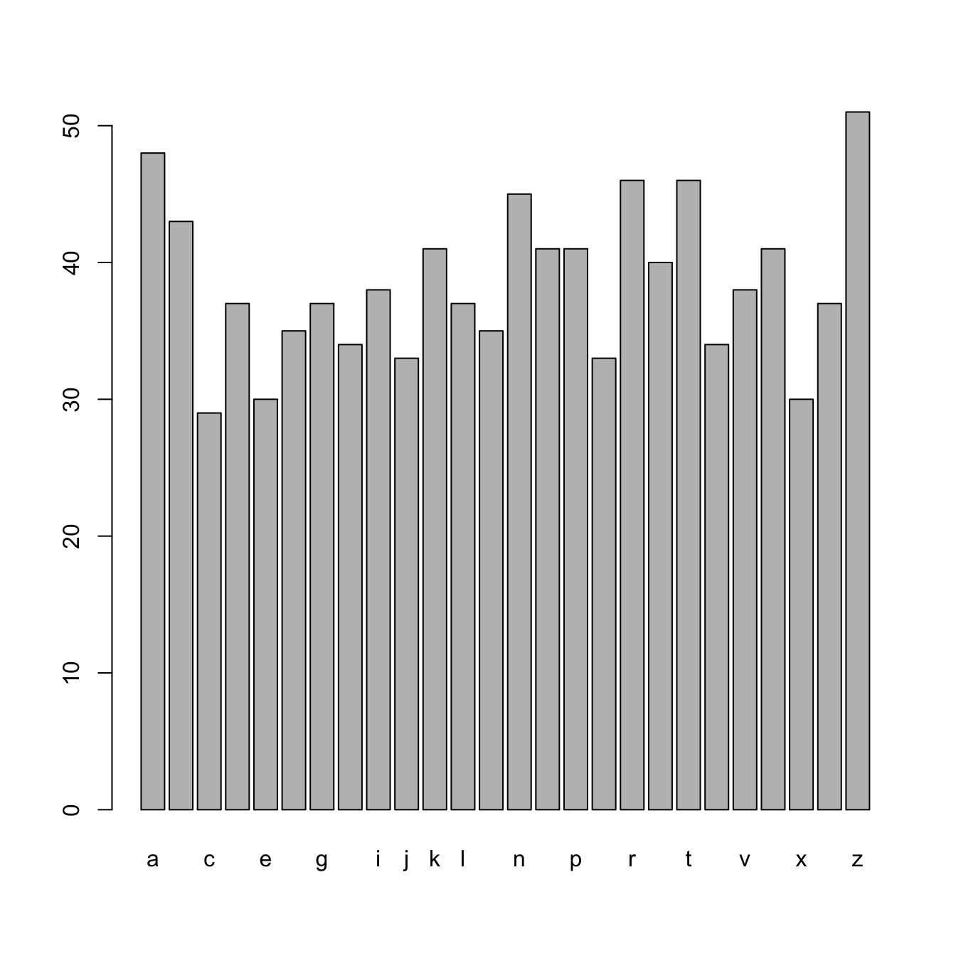
txtbarchart(x = let)## ++---------+---------+----------+---------+---------+----+
## 5 + * * +
## | * * * * * * |
## 4 + * * * * * * * * * * * * * +
## | * * * * * * * * * * * * * * * * * * * * * * * |
## 3 + * * * * * * * * * * * * * * * * * * * * * * * * * * +
## | * * * * * * * * * * * * * * * * * * * * * * * * * * |
## 2 + * * * * * * * * * * * * * * * * * * * * * * * * * * +
## | * * * * * * * * * * * * * * * * * * * * * * * * * * |
## 1 + * * * * * * * * * * * * * * * * * * * * * * * * * * +
## | * * * * * * * * * * * * * * * * * * * * * * * * * * |
## 0 + * * * * * * * * * * * * * * * * * * * * * * * * * * +
## ++---------+---------+----------+---------+---------+----+
## 0 5 10 15 20 25
## Legend:
## 1=a, 2=b, 3=c, 4=d, 5=e, 6=f, 7=g, 8=h, 9=i, 10=j, 11=k, 12=
## l, 13=m, 14=n, 15=o, 16=p, 17=q, 18=r, 19=s, 20=t, 21=u, 22=
## v, 23=w, 24=x, 25=y, 26=z# txtcurve
curve(expr = sin(x), from = 0, to = 2 * pi)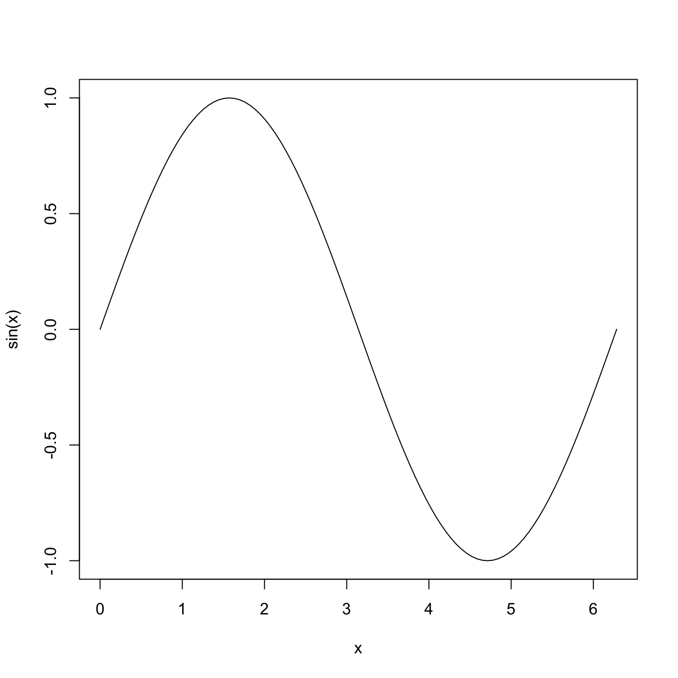
txtcurve(expr = sin(x), from = 0, to = 2 * pi)## +-+-------+-------+-------+-------+------+-------+----+
## 1 + ********* +
## | *** *** |
## | ** ** |
## 0.5 + ** ** +
## | ** ** |
## | * * |
## 0 + * ** ** +
## | ** ** |
## -0.5 + ** * +
## | ** ** |
## | *** *** |
## -1 + ********* +
## +-+-------+-------+-------+-------+------+-------+----+
## 0 1 2 3 4 5 6# txtacf
acf(x)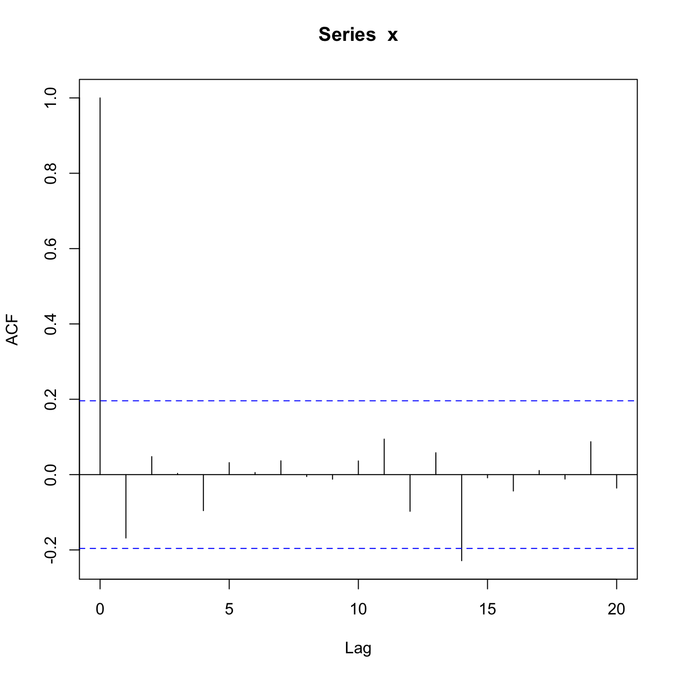
txtacf(x)## +-+------------+-----------+-----------+-----------+--+
## 1 + * +
## | * |
## 0.8 + * +
## 0.6 + * +
## | * |
## 0.4 + * +
## | * |
## 0.2 + * +
## | * * * |
## 0 + * * * * * * * * * * * * * * * * * * * * * +
## | * * * * * * |
## -0.2 + * * +
## +-+------------+-----------+-----------+-----------+--+
## 0 5 10 15 20library(NostalgiR) # nos.* functions
# Mexican hat
xx <- seq(-10, 10, l = 50)
yy <- xx
f <- function(x, y) {r <- sqrt(x^2 + y^2); 10 * sin(r)/r}
zz <- outer(xx, yy, f)
# nos.density
plot(density(x)); rug(x)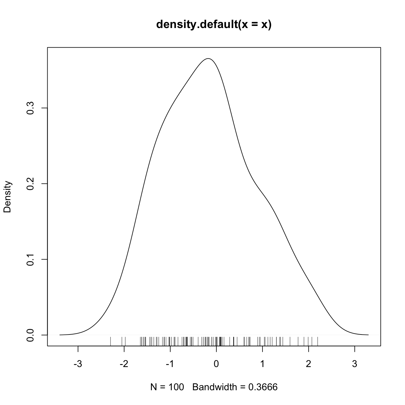
nos.density(x)## +-----------+--------------+-------------+-----------+
## | ~~~~~~ |
## | ~~~ ~~ |
## 0.3 + ~~~ ~~ +
## D | ~~ ~~ |
## e | ~~ ~~ |
## n 0.2 + ~~ ~~~ +
## s | ~~ ~~~ |
## i | ~~ ~~ |
## t 0.1 + ~~ ~~~ +
## y | ~~ ~~~ |
## | ~~~ ~~~ |
## 0 + ~~~~~~~~o oo oooooooooooooooooooooooo oooo~~~~~~~ +
## +-----------+--------------+-------------+-----------+
## -2 0 2# nos.hist
hist(x)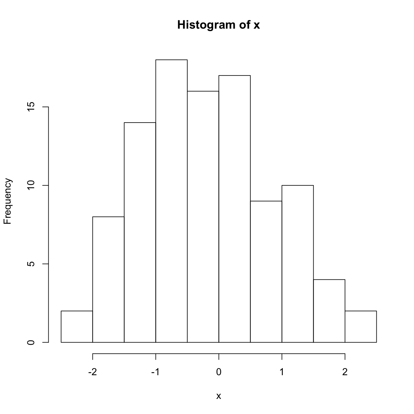
nos.hist(x)## +----+----------+----------+----------+----------+----+
## | o o |
## | o o o |
## F 15 + o o o o +
## r | o o o o |
## e | o o o o |
## q 10 + o o o o o +
## u | o o o o o o o |
## e | o o o o o o o |
## n 5 + o o o o o o o +
## c | o o o o o o o o |
## y | o o o o o o o o o o |
## 0 + o o o o o o o o o o +
## +----+----------+----------+----------+----------+----+
## -2 -1 0 1 2# nos.ecdf
plot(ecdf(x))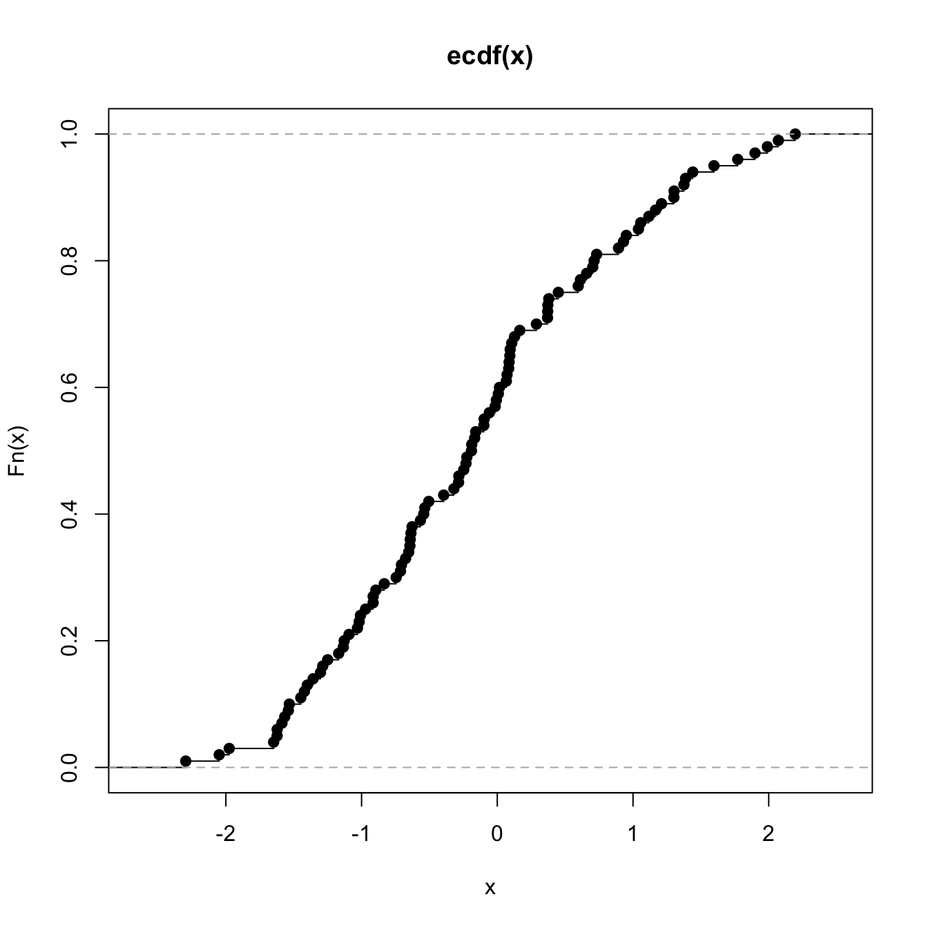
nos.ecdf(x)## +-----+---------+----------+----------+---------+----+
## 1 + o~o~ooooo +
## | ooooo |
## 0.8 + ooo~o~ +
## | ooooo~ |
## E 0.6 + oo +
## C | ooo |
## D | ooo |
## F 0.4 + ooo~ +
## | oooo |
## 0.2 + oooo +
## | ooooo |
## | o~~oo~~oo |
## 0 +-----+---------+----------+----------+---------+----+
## -2 -1 0 1 2# nos.qqnorm
qqnorm(x); qqline(x)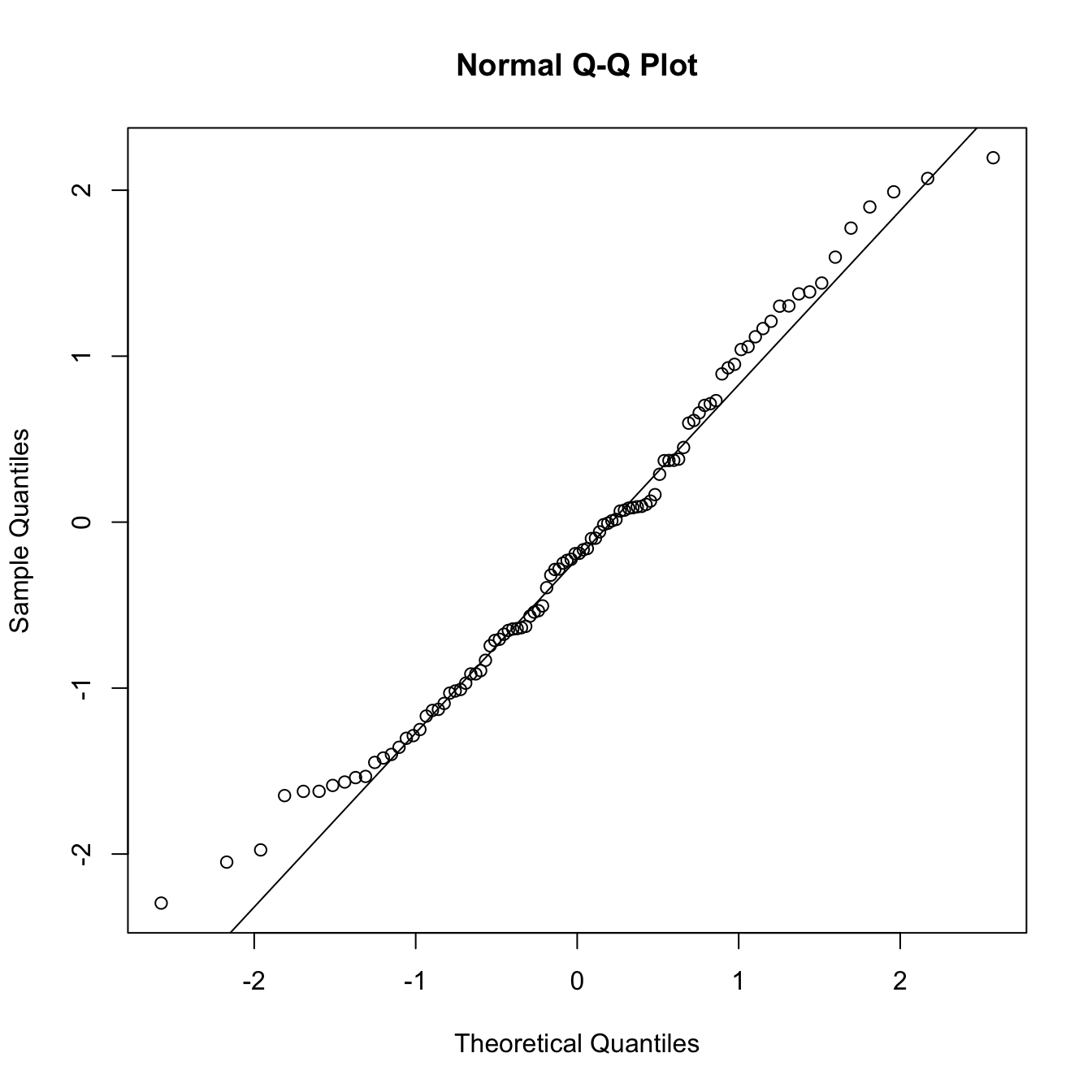
nos.qqnorm(x)## +-------+--------+---------+--------+---------+-------+
## 2 + o~o~o~ o +
## S | ooo~~ |
## a 1 + ooooo +
## m | ooo~ |
## p | ~~oo~ |
## l 0 + oooooo +
## e | oooo |
## -1 + ooooo +
## Q | ooooo |
## s | ooooo |
## -2 + o o~o~~~ +
## +-------+--------+---------+--------+---------+-------+
## -2 -1 0 1 2
## Theoretical Qs# nos.qqplot
qqplot(x, y)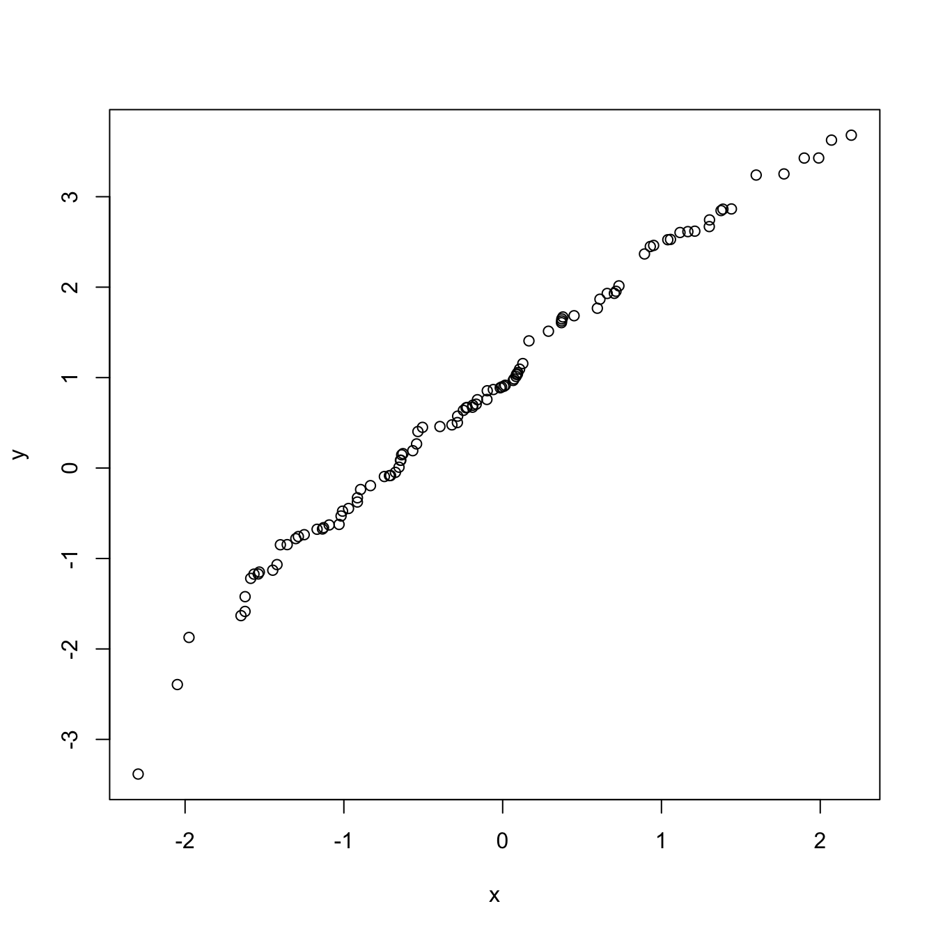
nos.qqplot(x, y)## 4 +-----+----------+-----------+----------+----------+----+
## | o ooooo |
## | ooooo |
## 2 + o oo ~~~ +
## | o ooooo ~~~~~~~ |
## | oooo ~~~~~~~~ |
## | ooooooo ~~~~~~~~ |
## 0 + oooo ~~~~~~~ +
## | oooooo~~~~~ |
## | ooo~~~~~ |
## -2 + ~~~o~~~~ +
## | ~ o |
## | o |
## +-----+----------+-----------+----------+----------+----+
## -2 -1 0 1 2# nos.contour
contour(xx, yy, zz)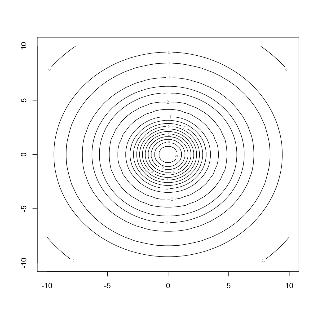
nos.contour(data = zz, xmin = min(xx), xmax = max(xx),
            ymin = min(yy), ymax = max(yy))
## +-+------------+-----------+------------+-----------+--+
## 10 + 33 22 22222 3333333333 22222 222 33 +
## | 33332222222233333444444444444443333322222222333 |
## | 333222 222333444444 444444333222 22233 |
## | 222222333444 444444444444444444 444333222222 |
## 5 + 2 22233444 44443333222222222233334444 4443322 2 +
## | 2 3344 444332 1111111111111111 233444 4433 2 |
## | 22 3 44 44332111112345555554321111123344 44 3 2 |
## | 3 44 4332 111134555 555431111 2334 4433 |
## | 3 4 4 32 111 245 542 11 2344 4 3 |
## 0 + 3 4 4 32 111 245 542 11 2344 4 3 +
## | 3 44 4332 111134555 555431111 2334 4433 |
## | 22 3 44 43322111112345555554321111122344 44 3 2 |
## | 2233344 444332111111111111111111233444 4433322 |
## -5 + 2 22233444 44443332222111122223334444 4443322 2 +
## | 222222333444 444444444444444444 444333222222 |
## | 333222 222333444444 444444333222 22233 |
## | 3333222 22223333344444444444444333332222 222333 |
## -10 + 33 222 22222 3333333333 22222 2222 33 +
## +-+------------+-----------+------------+-----------+--+
## -10 -5 0 5 10
## Legend: 1 ~ -2.02; 2 ~ -0.769; 3 ~ -0.082; 4 ~ 0.795; 5 ~ 1.74# nos.image
image(zz, col = viridis(50))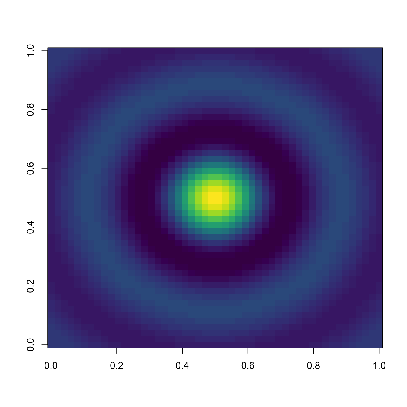
nos.image(data = zz, xmin = min(xx), xmax = max(xx),
          ymin = min(yy), ymax = max(yy))
## +-+------------+-----------+------------+-----------+--+
## 10 + o oooo........................................ooooo +
## | o oo....................oooo....................ooo |
## | . .............oooooooooooooooooooooo.............. |
## | . .........oooooooooooooooooooooooooooooo.......... |
## 5 + . ......oooooooooo................oooooooooo....... +
## | . ....oooooooo........................oooooooo..... |
## | . ...oooooooo..........................oooooooo.... |
## | . ..ooooooo..........oooxxxxooo..........ooooooo... |
## | . ..oooooo.........ooxXX####XXxoo.........oooooo... |
## 0 + . .ooooooo........ooxXX######XXxoo........ooooooo.. +
## | . ..ooooooo........ooxxXXXXXXxxoo........ooooooo... |
## | . ..oooooooo..........oooooooo..........oooooooo... |
## | . ...oooooooo..........................oooooooo.... |
## -5 + . .....oooooooo......................oooooooo...... +
## | . .......ooooooooooo............ooooooooooo........ |
## | . ..........oooooooooooooooooooooooooooo........... |
## | o ...............oooooooooooooooooo...............o |
## -10 + o ooo..........................................oooo +
## +-+------------+-----------+------------+-----------+--+
## -10 -5 0 5 10
## Legend:
## . ~ (-2.17,0.235); o ~ (0.235,2.64); x ~ (2.64,5.05); X ~ (5
## .05,7.45); # ~ (7.45,9.86)Cute animals with cowsay
cowsay is a package for printing messages with ASCII animals. Although it has little practical use, it is way fun! There is only one function, say, that produces an animal with a speech bubble.
library(cowsay)

# Random fortune
set.seed(363)
say("fortune", by = "random")
## Colors cannot be applied in this environment :( Try using a terminal or RStudio.
##
##  -----
## If 'fools rush in where angels fear to tread', then Bayesians 'jump' in where frequentists fear to 'step'.
##  Charles C. Berry
##  about Bayesian model selection as an alternative to stepwise regression
##  R-help
##  November 2009
##  ------
##     \
##      \
##       \
##        /\___/\
##        {o}{o}|
##        \ v  /|
##        |    \ \
##         \___/_/       [ab]
##           | |

# All animals
# sapply(names(animals), function(x) say(x, by = x))

# Annoy the users of your package with good old clippy
say(what = "It looks like you\'re writing a letter!",
    by = "clippy", type = "warning")
## Colors cannot be applied in this environment :( Try using a terminal or RStudio.
## Warning in say(what = "It looks like you're writing a letter!", by = "clippy", :
##
##  -----
## It looks like you're writing a letter!
##  ------
##     \
##      \
##    __
##    / \
##    | |
##    @ @
##   || ||
##   || ||
##   |\_/|
##   \___/ GB

# A message from Yoda
say("Participating in the Coding Club UC3M you must. Yes, hmmm.", by = "yoda")
## Colors cannot be applied in this environment :( Try using a terminal or RStudio.
##
##
##
##  -----
## Participating in the Coding Club UC3M you must. Yes, hmmm.
##  ------
##     \
##      \
##                    ____
##                 _.' :  `._
##             .-.'`.  ;   .'`.-.
##    __      / : ___\ ;  /___ ; \      __
##   ,'_ ""--.:__;".-.";: :".-.":__;.--"" _`,
##   :' `.t""--.. '<@.`;_  ',@>` ..--""j.' `;
##        `:-.._J '-.-'L__ `-- ' L_..-;'
##           "-.__ ;  .-"  "-.  : __.-"
##              L ' /.------.\ ' J
##              "-.   "--"   .-"
##              __.l"-:_JL_;-";.__
##          .-j/'.;  ;""""  / .'\"-.
##          .' /:`. "-.:     .-" .';  `.
##       .-"  / ;  "-. "-..-" .-"  :    "-.
##   .+"-.  : :      "-.__.-"      ;-._   \
##   ; \  `.; ;                    : : "+. ;
##   :  ;   ; ;                    : ;  : \:
##   ;  :   ; :                    ;:   ;  :
##   : \  ;  :  ;                  : ;  /  ::
##   ;  ; :   ; :                  ;   :   ;:
##   :  :  ;  :  ;                : :  ;  : ;
##   ;\    :   ; :                ; ;     ; ;
##   : `."-;   :  ;              :  ;    /  ;
##  ;    -:   ; :              ;  : .-"   :
##   :\     \  :  ;            : \.-"      :
##   ;`.    \  ; :            ;.'_..--  / ;
##   :  "-.  "-:  ;          :/."      .'  :
##    \         \ :          ;/  __        :
##     \       .-`.\        /t-""  ":-+.   :
##      `.  .-"    `l    __/ /`. :  ; ; \  ;
##        \   .-" .-"-.-"  .' .'j \  /   ;/
##         \ / .-"   /.     .'.' ;_:'    ;
##   :-""-.`./-.'     /    `.___.'
##                \ `t  ._  /  bug
##                 "-.t-._:'
##