An introduction to Shiny as a teaching resource

Antonio Elías Fernández

Tue, Jun 19, 2018 19 min read R Source

The main goal of this session is to show a regular R user how to develop his/her own interactive (web) application without much effort. For doing so, we introduce the Shiny R package that makes this task simple even for an R programmer that has never heard about HTML, CSS or JavaScript (or does not care about them at all). During the session, we will develop from scratch an interactive app that illustrates the law of large numbers. This will allow us to understand the input and output of a Shiny app, as well as the whole workflow intuition for building Shiny apps.

We will need RStudio with R (>= 3.0.2) and the following package:

install.packages("shiny", dependencies = TRUE)

Introduction

New teaching methodologies have arised during the last years and many of them have been leaded by the introduction of emerging technologies. Bright examples are Active Learning or Research-Informed Learning phylosophies which aim to give a more participative role to the students and motivates the learning proccess by means of practical examples.

In addition to be a pontetially more enjoyable approach, these methodologies have demostrated to improve significanly the performance of the students in many areas of knowledge in high level education. Freeman et Al (2014) compared the performance in undergraduate science, technology, engineering, and mathematics courses under traditional lecturing versus Active Learning and concluded that “average examination scores improved by about 6% in Active Learning sections, and that students in classes with traditional lecturing were 1.5 times more likely to fail than were students in classes with Active Learning”. As another example, Fawcett (2018) introduced Interactive Shiny Apps for supporting Research-Informed Learning and Teaching. They studied its effect on students’ responses in data analysis work, and assigments that require the interpretation of methods in a recently published paper. For doing so, they compare the results of student who had access to the Apps versus student that did not and they concluded that the methods benefited students, not only in terms of their ability to understand and implement advanced techniques from the recent literature but also in terms of their confidence and overall satisfaction with the course. In the same direction, Williams and Williams (2017) and Doi et al (2016) used R Shiny App as support for their innovation teaching projects.

Universities and academic staff have noticed the potencial of such as Shiny R Applications as a teaching tool and they have put effort on developing repositories with examples in different topics.

Despite the main motivation of the session is devoted to teaching and researching, Shiny App is becoming more and more employed in industry. Their usefulness and adaptability to different needs do not have limit as can be shown in these more ambicious examples and these others.

What is an Interactive Web R Shiny App?

What is a Web?

A web page is just a set of files HTML (HyperText Markup Language), CSS (Cascading Style Sheets) and JS (JavaScript) typically located in a server. We, as users, can request these data from our computer and display them with a browser. This process is outlined in the figure below.

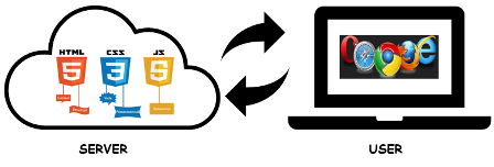
Each of this files enumarated above has a different goal. HTML is in charge of including the information we want to visualize and building the structure of the web. CSS introduces the desing of the web and how to present the information. Finally, JS is the programming lenguage of HTML and allows to introduce dynamics.

As the abstracts says, today we do not need knowledge about these but it is important to take it into account to value the work that Shiny is doing for us. Despite this, basic knowledge of web programming would increase exponentially your options.

What is an Interactive App?

The user can interactuate with the server in such a way he/she can lead the process behind the App. The user declare input or variables that the developer design for being modificated by him/her. Afterwards, the server uses this input for conditionally returning the output.

This trade off between user and server is a key point and it is the difference between a dynamic App and a static document (.pdf) or a book. The following diagram illustrates this workflow for an App runing on a server.

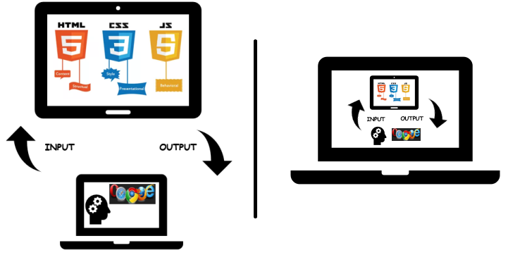
Today we will forget about the comunication betwen user and server and our dynamic App will be running locally; the user and the files providing the web are in the same place as at the right panel of the sketch above.

What is R Shiny?

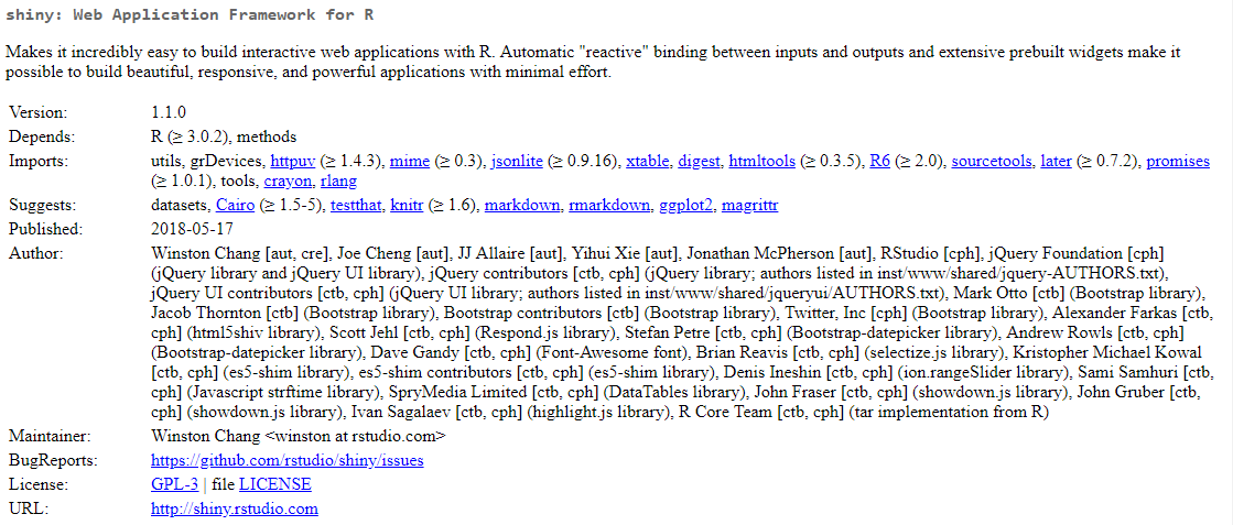
The Shiny package in CRAN is a web application framework for R. Obviously, the idea of creating an application with statistical purposes is not new at all, in fact, there are many projects related with the development of Applet. However, this tool require high knowledge of web programming, while Shiny mitigates this drawback by nesting R functions that assemble a complete Application.

Developing a Shiny App

Baselines

In this section, we present a simple template with the skeleton of a Shiny App. It can be taken as a starting point for developing any other App. Mainly, it contains the following parts:

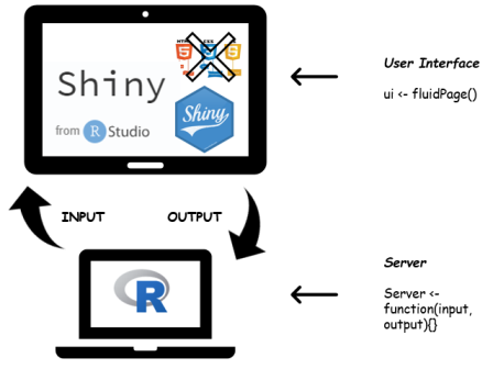
ui (User Interface) - nested R functions that assemble an HTML user interface for the App. Is is in charge of the contents and style of the App,
server - a function with instructions on how to build and rebuild the R objects displayed in the UI. Its arguments are the inputs and the outputs of the App. In this part is where our R code is going to be included.
shinyApp - combines ui and server into an App.

library('shiny')

ui <- fluidPage(content1, content2,...)

server <- function(input, output){}

shinyApp(ui = ui, server = server)

As the diagram below shows, the input and ouput trade off plays the role of being the communication link between user and server. In addition to that, thanks to the Shiny package, one could avoid web programming and simply install the package in a machine with RStudio.

Once we have understood the main workflow, we are going to develope an App from a simple R code. From my point view, a good strategy for building a Shiny R App is to thing about our R code in terms of input and ouput objects. In other words, what we want to be choosen by the user and what we want to show to the user given his/her inputs selection. As an illustration, we are going to build a Shiny App based on the next code that empirically demonstrates the Law of Large Numbers. For the moment, let us consider $N$ realizations of a $X\sim Bern(p)$, then sample mean $\sum_{i=1}^N \frac{x_i}{N} \rightarrow E[X]=p$ as $N \rightarrow \infty$.

The code below shows a bar plot of the realization, a cumulative mean plot versus the number of realizations and some statistics.

N <- 1000 # Number of realizations
p <- 0.25 # Parameter of the Bernouilli distribution
x <- rbinom(N, 1, p) # Binomial ~ Bin(n=1, p) == Bernouilli ~ Ber(p) 

par(mfrow = c(1, 2))
barplot(table(x)/N, ylim = c(0,1), ylab='Frecuency', main = 'Barplot')
plot(cumsum(x)/c(1:N), type = 'l', ylab = 'Y', xlab = 'Trials', main = 'LLN')
abline(h = p)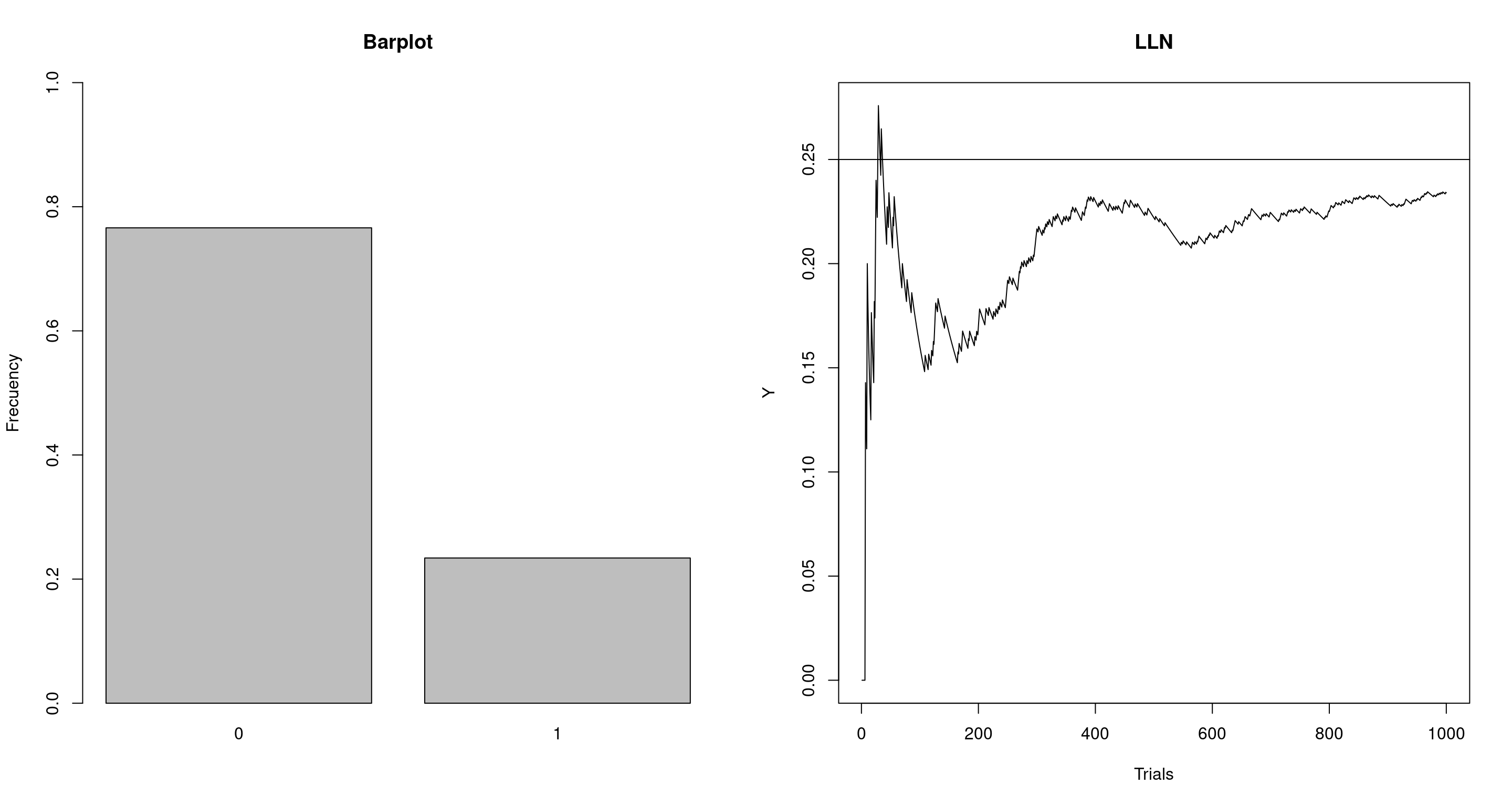

summary(x)

##    Min. 1st Qu.  Median    Mean 3rd Qu.    Max. 
##   0.000   0.000   0.000   0.243   0.000   1.000

Which values from our code are going to be inputs and which one outputs?

Inputs Objects

In orther to see that the empirical mean converges to the expected value, one would like to see how this sample mean behave when increasing the number of realizations $N$. In the same way, one could also think about modifiying the parameter $p$ of the distribution. Therefore, we have two inputs values i.e. $p$ and $N$.

There are many different functions from Shiny that allows to collect these values from the user. In the following figure, we have a set of examples:

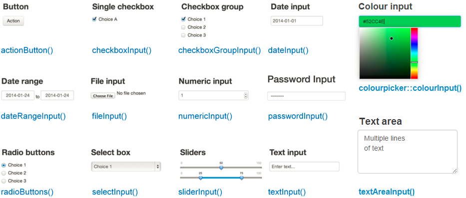
From Rbloggers Rblogger posts

These functions work as easy as a regular R function does and one could check their Description, Usage and Arguments by help('<functionName>'). However, the key point here is to answer the following question: must this chunk of code be at the UI or in the server part of our template?

help('numericInput')
help('sliderInput')

Among others, the most important and common argument in input functions is the inputId. It is the name that will allow us to access to the declared current input value by input$<inputId>.

library('shiny')

ui <- fluidPage(
  numericInput(inputId = 'N', "Sample Size", min = 1, max = 10000,  value = 10),
  sliderInput(inputId = 'p', "P( X = 1 )", min = 0, max = 1, value = 0.5),
  textInput(inputId = 'title', label = 'Write a label', value = 'Plot')
)

server <- function(input, output){}

shinyApp(ui = ui, server = server)

Output Objects

Once we have the input values, we can use them to produce an output with R for being provided to the user in the interface. This last sentence has two parts 1) to produce and 2) to provide in the same way we have to program our App by 1) render*() and 2) *Output() functions.

This two functions work together and each output function has its own render function counterpart. The following image presents some of this functions,

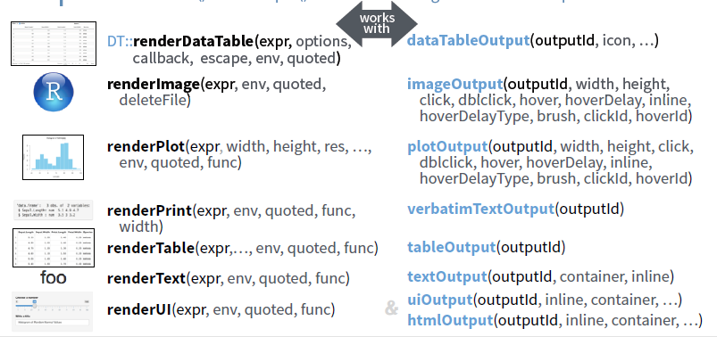
From Shiny Cheat Sheet

But one more time: must these chunks of code be at the UI, at the server part of our template?

help('renderPlot')
help('plotOutput')
help('verbatimTextOutput')

This trade off between render*() and *Output() functions is a cornerstone of reactivity. The server part would involve output$<myOutput> <- render*(expr,...), it produces the desired R ouput and it contains the R code in expr. Then, the output can be called from the UI by *Output(outputId = '<myOutput>').

library('shiny')

ui <- fluidPage(
  numericInput(inputId = 'N', "Sample Size", min = 1, max = 10000,  value = 10),
  sliderInput(inputId = 'p', "P( X = 1 )", min = 0, max = 1, value = 0.5),
  textInput(inputId = 'title', label = 'Write a label', value = 'Plot'),
  plotOutput(outputId = 'LLN'),
  verbatimTextOutput(outputId = 'stats')
)

server <- function(input, output){
  output$LLN <- renderPlot({
    x <- rbinom(input$N, 1, input$p)
    
    par(mfrow = c(1, 2))
    barplot(table(x)/input$N, ylim = c(0, 1), ylab = 'Frecuency')
    plot(cumsum(x)/c(1:input$N), type = 'l', ylab = 'Y', xlab = 'Trials', main = input$title)
    abline(h = input$p)
  })
  
  output$stats <- renderPrint({
    summary(rbinom(input$N, 1, input$p))
  })
}

shinyApp(ui = ui, server = server)

Modulating Reactivity

Up to here, we have desing very simple reactive relationship; each input is linked with a simple ouput. However, Shiny allows to have more complex connections through different functions. Some of them are the following,

reactive(): this function generate a reactive expression i.e. each time one its inputs values is modified, all its code is re-run. Once we have created the reactive value example <- reactive({code}), you can use the result by example().

What data set are the summary and the plot describing?

library('shiny')

ui <- fluidPage(
  numericInput(inputId = 'N', "Sample Size", min = 1, max = 10000,  value = 10),
  sliderInput(inputId = 'p', "P( X = 1 )", min = 0, max = 1, value = 0.5),
  textInput(inputId = 'title', label = 'Write a label', value = 'Plot'),
  plotOutput(outputId = 'LLN'),
  verbatimTextOutput(outputId = 'stats')
)

server <- function(input, output){
  
  data <- reactive({rbinom(input$N, 1, input$p)})
  
  output$LLN <- renderPlot({

    par(mfrow = c(1,2))
    barplot(table(data())/input$N, ylim = c(0, 1), ylab='Frecuency')
    plot(cumsum(data())/c(1:input$N), type = 'l', ylab = 'Y', xlab = 'Trials', main = input$title)
    abline(h = input$p)

  })
  
  output$stats <- renderPrint({
    summary(data())
  })
}

shinyApp(ui = ui, server = server)

isolate(): If we change any input object the code is rightaway completely re-run. We can isolate some input values in such a way the code is not re-run when modified but, of course, its effect will be taken into account.

Each time we modified the title we obtain a new data set. Can we isolate changes in the title of the plot?

library('shiny')

ui <- fluidPage(
  numericInput(inputId = 'N', "Sample Size", min = 1, max = 10000,  value = 10),
  sliderInput(inputId = 'p', "P( X = 1 )", min = 0, max = 1, value = 0.5),
  textInput(inputId = 'title', label = 'Write a label', value = 'Plot'),
  plotOutput(outputId = 'LLW'),
  verbatimTextOutput(outputId = 'stats')
)

server <- function(input, output){
  output$LLW <- renderPlot({
    x <- rbinom(input$N, 1, input$p)
    
    par(mfrow = c(1, 2))
    barplot(table(x)/input$N, ylim = c(0, 1), ylab = 'Frecuency')
    plot(cumsum(x)/c(1:input$N), type = 'l', ylab = 'Y', xlab = 'Trials', main = isolate(input$title))
    abline(h = input$p)
  })
  
  output$stats <- renderPrint({
    summary(x)
  })
}

shinyApp(ui = ui, server = server)

Triggers: One could also introduce action buttoms in our UI, actionButtom(), for controling the moment when the code reacts to an input change by using observeEvent(). There is also an observe({}) that will re-run all the code inside its {} if any of its inputs are modified, it is a reactive function.

library('shiny')

ui <- fluidPage(
  numericInput(inputId = 'N', "Sample Size", min = 1, max = 10000,  value = 10),
  sliderInput(inputId = 'p', "P( X = 1 )", min = 0, max = 1, value = 0.5),
  textInput(inputId = 'title', label = 'Write a label', value = 'Plot'),
  actionButton(inputId ='go', label='Go'),
  plotOutput(outputId = 'LLW'),
  verbatimTextOutput(outputId = 'stats')
)

server <- function(input, output){
  observeEvent(input$go, {
    output$LLW <- renderPlot({
      x <- rbinom(input$N, 1, input$p)
      
      par(mfrow = c(1, 2))
      barplot(table(x)/input$N, ylim = c(0, 1), ylab = 'Frecuency')
      plot(cumsum(x)/c(1:input$N), type = 'l', ylab = 'Y', xlab = 'Trials', main = input$title)
      abline(h = input$p)
    })
    
    output$stats <- renderPrint({
      summary(rbinom(input$N, 1, input$p))
    })
  }
  
  )
}

shinyApp(ui = ui, server = server)

Delay actions: we could also include a bottom that trigger reactive values just when clicked. rv <- eventReactive( input$go, {rnorm}).
Creating your own list of reactive values with rv <- reativeEvent(data = , ...) that can be overwritten if some event is observed with observeEvent(input$go, {rv$data = other data}).

library('shiny')

ui <- fluidPage(
  numericInput(inputId = 'N', "Sample Size", min = 1, max = 10000,  value = 10),
  sliderInput(inputId = 'p', "P( X = 1 )", min = 0, max = 1, value = 0.5),
  plotOutput(outputId = 'LLN'),
  verbatimTextOutput(outputId = 'stats')
)

server <- function(input, output){
  
  data <- reactive({
    rbinom(input$N, 1, input$p)
  })
  
  output$LLN <- renderPlot({
    par(mfrow = c(1, 2))
    barplot(table(data())/input$N, ylim = c(0, 1), ylab = 'Frecuency')
    plot(cumsum(data())/c(1:input$N), type = 'l', ylab = 'Y', xlab = 'Trials')
    abline(h = input$p)
  })
  
  output$stats <- renderPrint({
    summary(data())
  })
}

shinyApp(ui = ui, server = server)

Some of this functions may appear so similar in this when applying to our example. However, each one satisfies one different need for more complex settings.

Polishing our App

Up to here, we have just messed inputs and ouputs up without any structure at all. Now is the moment for making up our App and arranging the contents in a friendly and beautiful structure.

As explained at the beginning, the UI part of the code is in charge of the visualization aspect and therefore all the code related with these will be located at the fluidPage() function.

Adding layouts

One possible option is to organize our input and output with layout functions. In the figure below, we have som examples.

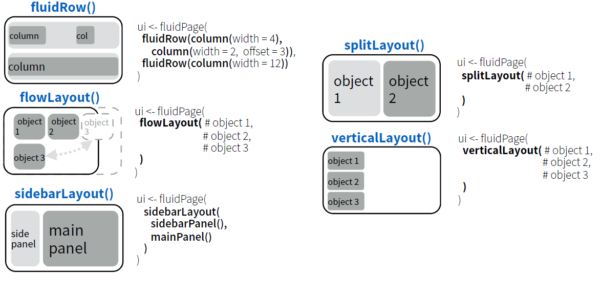
From Shiny https://www.rstudio.com/resources/cheatsheets/

For our Shiny App example, we can define the layout with sidebarLayout() as follows,

library('shiny')

ui <- fluidPage(
  sidebarLayout(
    sidebarPanel(
      numericInput(inputId = 'N', "Sample Size", min = 1, max = 10000,  value = 10),
      sliderInput(inputId = 'p', "P( X = 1 )", min = 0, max = 1, value = 0.5),
      textInput(inputId = 'title', label = 'Write a label', value = 'Plot')
    ),
    mainPanel(   
      plotOutput(outputId = 'LLN'),
      verbatimTextOutput(outputId = 'stats')
    )
  )
)

server <- function(input, output){
  
  data <- reactive({rbinom(input$N, 1, input$p)})
  
  output$LLN <- renderPlot({

    par(mfrow = c(1, 2))
    barplot(table(data())/input$N, ylim = c(0, 1), ylab='Frecuency')
    plot(cumsum(data())/c(1:input$N), type = 'l', ylab = 'Y', xlab = 'Trials', main = input$title)
    abline(h = input$p)

  })
  
  output$stats <- renderPrint({
    summary(data())
  })
}

shinyApp(ui = ui, server = server)

Adding tabs

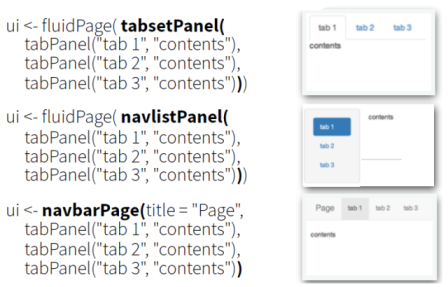
One could also structure the App in diffent panels with simple functions. From Shiny https://www.rstudio.com/resources/cheatsheets/

Lets suppose that we want to explit the different outputs in different tabs with tabsetPanel at our main panel layout section. And lets also add a table printing the generate data set.

library('shiny')

ui <- fluidPage(
  sidebarLayout(
    sidebarPanel(
      numericInput(inputId = 'N', "Sample Size", min = 1, max = 10000,  value = 10),
      sliderInput(inputId = 'p', "P( X = 1 )", min = 0, max = 1, value = 0.5),
      textInput(inputId = 'title', label = 'Write a label', value = 'Plot')
    ),
    mainPanel( 
      tabsetPanel(
        tabPanel('Plot', plotOutput(outputId = 'LLN')),
        tabPanel('Summary', verbatimTextOutput(outputId = 'stats')),
        tabPanel('Data', dataTableOutput(outputId = 'realization'))
      )
    )
  )
)

server <- function(input, output){
  
  data <- reactive({rbinom(input$N, 1, input$p)})
  
  output$LLN <- renderPlot({

    par(mfrow = c(1, 2))
    barplot(table(data())/input$N, ylim = c(0, 1), ylab = 'Frecuency')
    plot(cumsum(data())/c(1:input$N), type = 'l', ylab = 'Y', xlab = 'Trials', main = input$title)
    abline(h = input$p)

  })
  
  output$stats <- renderPrint({
    summary(data())
  })
  
  output$realization <- renderDataTable({
    tableAux <- cbind(1:input$N, data()); colnames(tableAux) <- c('Observation id', 'Realization')
    data.frame(tableAux)
  })
}

shinyApp(ui = ui, server = server)

UI is an HTML document!

Rstudio and Shiny converst our code inside fluidPage into a HTML file for builing our web App. One can observed this fact just by running the following code in the console,

library(shiny)

fluidPage(h1('Hello'))

fluidPage(headerPanel("Sliders"))

fluidPage(
  headerPanel("Sliders"),
  sidebarLayout(
    sidebarPanel(
    ),
    mainPanel( 
      tabsetPanel(
        tabPanel('tab1'),
        tabPanel('tab2'),
        tabPanel('tab3')
      )
    )
  )
)

The ouput is a translation of our Shiny R functions to their HTML counterparts. Then, one must suspect that is almost straighforward to add HTML code through tags. Moreover, it is also allowed to include CSS as well as JS files with includeCSS and includeScript.

library('shiny')

ui <- fluidPage(
  h1('HERE GOES MY APP'),
  sidebarLayout(
    sidebarPanel(
      numericInput(inputId = 'N', "Sample Size", min = 1, max = 10000,  value = 10),
      sliderInput(inputId = 'p', "P( X = 1 )", min = 0, max = 1, value = 0.5),
      textInput(inputId = 'title', label = 'Write a label', value = 'Plot')
    ),
    mainPanel( h2('Here we could include some comments about the App like'),
               h3('In probability theory, the law of large numbers (LLN) is a theorem that    describes the result of performing the same experiment a large number of times. According to the law, the average of the results obtained from a large number of trials should be close to the expected value, and will tend to become closer as more trials are performed.'),
      tabsetPanel(
        tabPanel('tab1', plotOutput(outputId = 'LLN')),
        tabPanel('tab2', verbatimTextOutput(outputId = 'stats')),
        tabPanel('tab3', dataTableOutput(outputId = 'realization'))
      )
    )
  ),
  includeCSS('mystyle.css')
)

server <- function(input, output){
  
  data <- reactive({rbinom(input$N, 1, input$p)})
  
  output$LLN <- renderPlot({

    par(mfrow = c(1, 2))
    barplot(table(data())/input$N, ylim = c(0, 1), ylab = 'Frecuency')
    plot(cumsum(data())/c(1:input$N), type = 'l', ylab = 'Y', xlab = 'Trials', main = input$title)
    abline(h = input$p)

  })
  
  output$stats <- renderPrint({
    summary(data())
  })
  
  output$realization <- renderDataTable({
    tableAux <- cbind(1:input$N, data()); colnames(tableAux) <- c('Observation id', 'Realization')
    data.frame(tableAux)
  })
}

shinyApp(ui = ui, server = server)

Other handy features

Conditional Panels

Following with our App, one could be willing to proof empirically the Law of Large Number but for a random variable coming from another distribution rather than Bernouilli. This task brings the problem of including inputs that depends on the selected distribution. In other words, one would need conditional panels. For example, if the selected distribution is the univariate Gaussian, one would like to have as input $\mu$ and $\sigma ^2$ rather than $p$.

Fortuntely, we can use the function conditionalPanel() in addition to an extra input object for selecting the distribution. For now, lets just include a binomial, $Bin(n,p)$ and an univariate Gaussian distribution, $N(\mu, \sigma)$.

library('shiny')

ui <- fluidPage(
  headerPanel("Law of Large Numbers"),
  sidebarLayout(
    sidebarPanel(
        selectInput('dist', 'Distribution', c("Bernoulli" = "bern", "Binomial" = "bin", "Normal" = 'norm'), selected = "bern"),
        conditionalPanel(
          condition = "input.dist == 'bern'",
          numericInput(inputId = 'Nsample', "Sample Size", min = 1, max = 10000,  value = 10),
          sliderInput(inputId = 'p', "P( X = 1 )", min = 0, max = 1, value = 0.5)
        ),
        conditionalPanel(
          condition = "input.dist == 'bin'",
          numericInput(inputId = 'Nsample2', "Sample Size", min = 1, max = 10000,  value = 10),
          sliderInput(inputId = 'trials', "Number Trials", min = 1, max = 1000, value = 1),
          sliderInput(inputId = 'p2', "P( X = 1 )", min = 0, max = 1, value = 0.5)
        ),
        conditionalPanel(
          condition = "input.dist == 'norm'",
          numericInput(inputId = 'Nsample3', "Sample Size", min = 1, max = 10000,  value = 10),
          numericInput(inputId = 'mu', "Mean", min = -1000, max = 1000, value = 0),
          sliderInput(inputId = 'sd', "Sd", min = 0, max = 1000, value = 1)
        )
    ),
    mainPanel(plotOutput(outputId = 'LLN'))
  )
)

server <- function(input, output){
  output$LLN <- renderPlot({
    if(input$dist == "bern"){
      x <- rbinom(input$Nsample, 1, input$p)
      par(mfrow = c(1,2))
      barplot(table(x)/input$Nsample, ylim=c(0,1), ylab = 'Frecuency')
      plot(cumsum(x)/c(1:input$Nsample), type='l', ylab='Y', xlab = 'Realization')
      abline(h=input$p)
    }
    if(input$dist == "bin"){
      x <- rbinom(input$Nsample2, input$trials, input$p2)
      par(mfrow = c(1, 2))
      barplot(table(x)/input$Nsample2, ylab = 'Frecuency')
      plot(cumsum(x)/c(1:input$Nsample2), type = 'l', ylab = 'Y', xlab = 'Realization')
      abline(h = input$p2*input$trials)
    }
    if(input$dist == "norm"){
      x <- rnorm(input$Nsample3, input$mu, input$sd)
      par(mfrow = c(1, 2))
      hist(x, ylab = 'Histogram')
      plot(cumsum(x)/c(1:input$Nsample3), type = 'l', ylab = 'Y', xlab = 'Realization')
      abline(h = input$mu)
    }
    
  })
}

shinyApp(ui = ui, server = server)

Shiny themes

We could also like to use a nice style but we do not want to include a CSS file. In this case, there are pre-defined themes with the package shinythemes.

library('shiny')
library('shinythemes')

ui <- fluidPage(theme=shinytheme("cosmo"),
  headerPanel("Law of Large Numbers"),
  sidebarLayout(
    sidebarPanel(
      selectInput('dist', 'Distribution', c("Bernoulli" = "bern", "Binomial" = "bin", "Normal" = 'norm'), selected = "bern"),
      conditionalPanel(
        condition = "input.dist == 'bern'",
        numericInput(inputId = 'Nsample', "Sample Size", min = 1, max = 10000,  value = 10),
        sliderInput(inputId = 'p', "P( X = 1 )", min = 0, max = 1, value = 0.5)
      ),
      conditionalPanel(
        condition = "input.dist == 'bin'",
        numericInput(inputId = 'Nsample2', "Sample Size", min = 1, max = 10000,  value = 10),
        sliderInput(inputId = 'trials', "Number Trials", min = 1, max = 1000, value = 1),
        sliderInput(inputId = 'p2', "P( X = 1 )", min = 0, max = 1, value = 0.5)
      ),
      conditionalPanel(
        condition = "input.dist == 'norm'",
        numericInput(inputId = 'Nsample3', "Sample Size", min = 1, max = 10000,  value = 10),
        numericInput(inputId = 'mu', "Mean", min = -1000, max = 1000, value = 0),
        sliderInput(inputId = 'sd', "Sd", min = 0, max = 1000, value = 1)
      )
    ),
    mainPanel(plotOutput(outputId = 'LLN'))
  )
)

server <- function(input, output){
  output$LLN <- renderPlot({
    if(input$dist == "bern"){
      x <- rbinom(input$Nsample, 1, input$p)
      par(mfrow = c(1,2))
      barplot(table(x)/input$Nsample, ylim=c(0,1), ylab = 'Frecuency')
      plot(cumsum(x)/c(1:input$Nsample), type='l', ylab='Y', xlab = 'Realization')
      abline(h=input$p)
    }
    if(input$dist == "bin"){
      x <- rbinom(input$Nsample2, input$trials, input$p2)
      par(mfrow = c(1, 2))
      barplot(table(x)/input$Nsample2, ylab = 'Frecuency')
      plot(cumsum(x)/c(1:input$Nsample2), type = 'l', ylab = 'Y', xlab = 'Realization')
      abline(h = input$p2*input$trials)
    }
    if(input$dist == "norm"){
      x <- rnorm(input$Nsample3, input$mu, input$sd)
      par(mfrow = c(1, 2))
      hist(x, ylab = 'Histogram')
      plot(cumsum(x)/c(1:input$Nsample3), type = 'l', ylab = 'Y', xlab = 'Realization')
      abline(h = input$mu)
    }
    
  })
}

shinyApp(ui = ui, server = server)

References

Scott Freeman, Sarah L. Eddy, Miles McDonough, Michelle K. Smith, Nnadozie Okoroafor, Hannah Jordt, and Mary Pat Wenderoth (2014). “Active Learning increases student performance in science, engineering, and mathematics”, PNAS. link
Fawcett, Lee (2018). “Using Interactive Shiny Applications to Facilitate Research-Informed Learning and Teaching”, Journal of Statistical Education. link
William, Immanuel James and William, Kelley Kim (2017). “Using an R shiny to enhance the learning experience of confidence intervals”, Teaching Statistics. link
Doi, Jimmipotter, Gailwong, Jimmyalcaraz and Irvinchi, Peter (2016). “Web Application Teaching Tools for Statistics Using R and Shiny”, Open Access Publication from the University of California, Center for the Teaching of StatisticsTechnology Innovations in Statistics Education. link

The materials of this session were mainly motivated by Shiny Tutorial and the following Rblogger posts.

R app shiny teaching