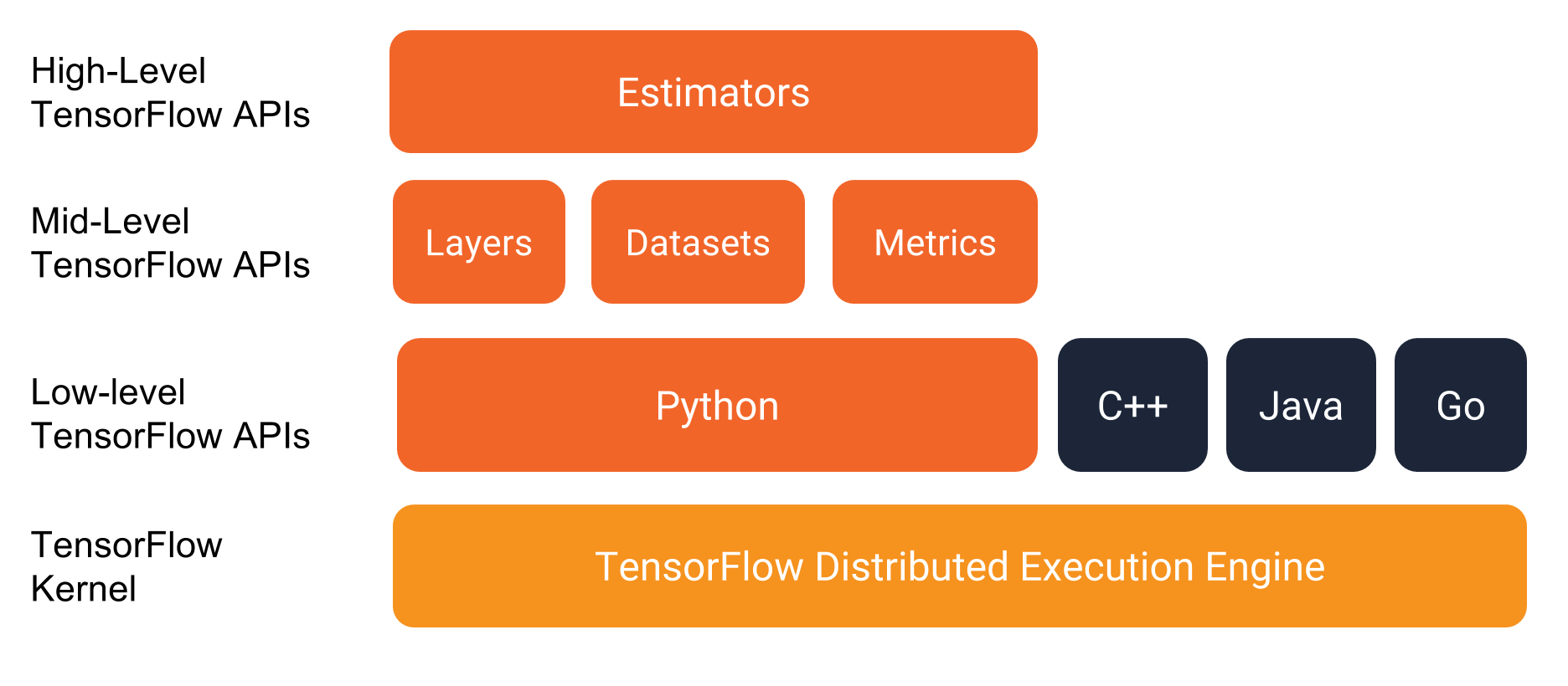
Tensorflow has been widely used for many applications in machine learning and deep learning. However, Tensorflow is more than that, it is a general purpose computing library. Based on that, people have created a rich ecosystem for quickly developing models. In this talk, I will show how statisticians can get most of the main features in Tensorflow such as automatic differentiation, optimization, and Bayesian analysis through a simple linear regression example.
Introduction
Tensorflow is a machine learning framework of Google. It is developed by Google Brain team since 2015 and released publicly in 02.2017. It is now implemented for many applications in machine learning and deep learning. It has API for Python, R, C.
Tensorflow is not only used for deep learning. As a statistician, there are a lot of features that we can take advantages.
- Tensorflow = general purpose computing library.
- Tensorflow in R = Interface to Tensorflow library.
- Computations are implemented as input data (tensor/ generalized matrix/ multidimensional array) flow through nodes (mathematical operators) to the output data.
Tensorflow features:
- Reverse-mode auto differentiation.
- Multicore CPU, GPU supports.
- Official Python API and C API, third-party packages for Julia, R.
- An ecosystem with numbers of machine learning algorithms
tfestimators,keras. - Graphical probabilistic modelling with
TensorFlow Probability. - Monitor and metrics with TensorBoard.

tensorflow
Install Tensorflow in R
We summary the main steps for installing Tensorflow package in R. For the full instruction, please go to:
Windows
Install python, pip3 and Tensorflow,
Download Python and install (Choose add path and install pip3).
Open cmd with administration role and execute,
pip3 install tensorflow==1.9.0rc1
pip3 install tfp-nightly==0.1.0rc1.dev20180702    # depends on tensorflow (CPU-only)
Ubuntu
- Install python, pip3 and Tensorflow,
sudo apt-get install python3-pip python3-dev
pip3 install tensorflow==1.9.0rc1
pip3 install tfp-nightly==0.1.0rc1.dev20180702    # depends on tensorflow (CPU-only)
macOS
Check pip3 version:
pip3 -V # for Python 3.nIf pip or pip3 8.1 or later is not installed, issue the following commands to install or upgrade:
sudo easy_install --upgrade pip
sudo easy_install --upgrade six
pip3 install tensorflow==1.9.0rc1
pip3 install tfp-nightly==0.1.0rc1.dev20180702    # depends on tensorflow (CPU-only)
Once you have installed Tensorflow, we go to RStudio and intall the R API package.
Install R package Tensorflow
install.packages("tensorflow", "reticulate")
tensorflow::install_tensorflow()
Hello Tensorflow
Test your installation with this chunk of codes
library(tensorflow)

sess <- tf$Session()

hello <- tf$constant("Hello, TensorFlow!")
sess$run(hello)

a <- tf$constant(10)
b <- tf$constant(32)
sess$run(a + b)

sess$close()
If everything works, we are ready to go.
TensorFlow API from R
We start with how to declare variables, constants and placeholders in Tensorflow.
We assign an object (sess) pointing to tf$Session()
and close a session with sess$close(). Here top level API is tf which provides access to Tensorflow modules.
There are several ways to evaluate a Tensorflow variable.
- Temporary use
tf$Session(),
tensor_0D <- tf$constant(42, name = "tensor_0D")    # Declare a constant
tensor_0D                                           # Print tensor

with(tf$Session() %as% sess, {      # temporary use tf$Session()
    sess$run(tensor_0D)             # Get the value of a tensor
})tf$Session()$run()intf$Session(),
 # Start a sesssion with tensorflow
sess <- tf$Session()
# vector of variables as a place holder
tensor_1D <- tf$Variable(c(1,2,3), name = "tensor_1D")
# Initiate the values of all variables ( include tensor_1D)
sess$run(tf$global_variables_initializer())
sess$run(tensor_1D)
sess$close() # Close a sessionobject_name$eval()intf$InteractiveSession(),
sess <- tf$InteractiveSession()             # An interactive session

# Data 2D : (samples, features)
tensor_2D <- tf$placeholder(tf$float32, c(2,4), name = "tensor_2D")
# Initialize tensor_2D with data
tensor_2D$eval(feed_dict = dict(tensor_2D = matrix(1:8, nrow = 2, ncol = 4)))


# 3D tensor variable
tensor_3D <- tf$Variable(tf$ones(c(3,2,2)), name = "tensor_3D")
sess$run(tf$global_variables_initializer()) # Initialize  all variables
tensor_3D$eval()                            # Instead of: sess$run(tensor_3D)
sess$close()                                # Close a session
tf$reset_default_graph()
Linear regression
Gradient descent algorithm
We analyze an example of simple linear regression to see how to use Tensorflow to optimize over a loss function. Then we use TensorBoard to monitor the loss function in each iteration. For a simple linear regression, we fit a linear function,
\[y = A x + b + \epsilon\]
such that it minimize the distance between the predicted values (\(\hat{y_i}\)) and the observed values (\(y_i\)) in term of mean square error.
\[MSE = \frac{1}{n} \sum_{i = 1}^n (y_i - \hat{y}_i)^2\]
In order to illustrate how to solve for this optimization, we use the iris data (collected by Ronald Fisher in his well-known 1936 paper).
We want to define a linear model between Petal.Length and Petal.Width.
We first create a placeholder (x_data, y_data) for (Petal.Length, Petal.Width),
Then, we derive the prediction \(\hat{y} = A x + b\).
# We model the relationship between Petal.Width and Petal.Length
data(iris)
#head(iris)
sess <- tf$Session()

x_data <- tf$placeholder(dtype = "float",
                         shape = length(iris$Petal.Length),
                         name = "Petal.Length") # Placeholder for Petal.Length
y_data <- tf$placeholder(dtype = "float",
                         shape = length(iris$Petal.Width),
                         name = "Petal.Width") # Placeholder for Petal.Width

A <- tf$Variable(0.0,   name = "Coefficient")
b <- tf$Variable(1.0,   name = "Intercept")

y_hat <- A * x_data + b
Secondly, we define a loss function (MSE) and a submodule optimizer tf$train$GradientDescentOptimizer
with a learning rate \(\gamma = 0.03\). There are several other submodules such as AdagradOptimizer, MomentumOptimizer, RMSPropOptimizer which based on the problem of interest. The GradientDescentOptimizer will update the parameters \(A\) and \(b\) in each iteration by,
\[A_{n+1} = A_{n} - \gamma \nabla MSE(A_n)\]
# Define MSE as the equation above
MSE <- tf$reduce_mean((y_data - y_hat)^2)
# Optimizer engine
optimizer <- tf$train$GradientDescentOptimizer(0.03)
# Define the objective function
train <- optimizer$minimize(MSE)
Finally, we fetch data to placeholder using feed_dict and update paramters along the gradient few thousand times.
sess$run(tf$global_variables_initializer()) # To init all the variables

for (epoch in 1:2000) {
        sess$run(train, feed_dict = dict(x_data = iris$Petal.Length,
                                       y_data = iris$Petal.Width))
}
cat("Coefficient: ", sess$run(A), "\n Intercept: ", sess$run(b), "\n")
sess$close()
tf$reset_default_graph()
# Compare to linear regression
lm(Petal.Width ~ Petal.Length, data = iris)Monitoring with TensorBoard
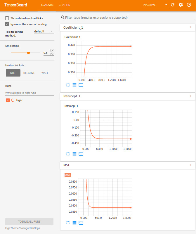
TensorBoard is a metrics module that helps to monitor the learning process. In the complex model, TensorBoard not only visualizes but also debug, optimize the objective function. Most of the codes in this section are inherited from the previous section with few lines for adding variables to our watch list.
# We model the relationship between Petal.Width and Petal.Length
data(iris)
#head(iris)

sess <- tf$Session()

x_data <- tf$placeholder(dtype = "float",
                         shape = length(iris$Petal.Length),
                         name = "Petal.Length") # Placeholder for Petal.Length
y_data <- tf$placeholder(dtype = "float",
                         shape = length(iris$Petal.Width),
                         name = "Petal.Width")  # Placeholder for Petal.Width

A <- tf$Variable(0.0,   name = "Coefficient")
b <- tf$Variable(1.0,   name = "Intercept")

y_hat <- A * x_data + b

MSE <- tf$reduce_mean((y_data - y_hat)^2)
optimizer <- tf$train$GradientDescentOptimizer(0.03)
train <- optimizer$minimize(MSE)

###########################################
# Add variable to summary #
# https://www.tensorflow.org/programmers_guide/summaries_and_tensorboard
###########################################
MSE_hist <- tf$summary$scalar("MSE", MSE)   # save all values of MSE
A_hist <- tf$summary$scalar("Coefficient", A)
b_hist <- tf$summary$scalar("Intercept", b)
merged <- tf$summary$merge_all()            # Merges all summaries collected in the default graph.

train_writer <- tf$summary$FileWriter(logdir = "/home/hoanguc3m/logs")
train_writer$add_graph(sess$graph)          # add a graph structure

###########################################
# End of summary #
###########################################

sess$run(tf$global_variables_initializer())

for (epoch in 1:2000) {
    result <- sess$run(list(merged, train),   # remember to run merged
                       feed_dict = dict(x_data = iris$Petal.Length,
                                      y_data = iris$Petal.Width))
    summary <- result[[1]]                    # extract the summary result of merged
    train_writer$add_summary(summary, epoch)  # write summary to disk
}

# cat("Coefficient: ", sess$run(A), "\n Intercept: ", sess$run(b), "\n")
sess$close()
tf$reset_default_graph()
rm(list = ls())
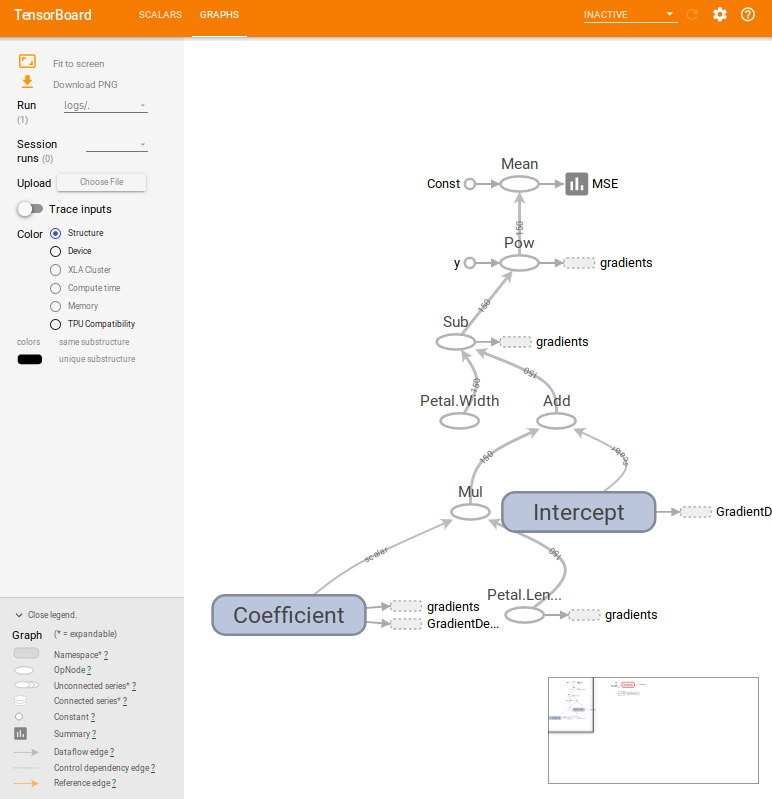
tensorboard(log_dir = "/home/hoanguc3m/logs") # Play with tensorboardHere are few things that we summary in TensorBoard. The algorithm reachs convergence after 1000 iterations. For graph structure, each node in the graph represents for an operator at the edge, we can see the flow of the data. It could be a scalar in case of \(A\) and \(b\) or it could be a vector in case of \(x\) and \(y\).


tensor_board
Maximum likelihood with Tensorflow
Tensorflow contains a large collection of probability distributions. tf$contrib$distributions provides some common distribution such as Bernoulli, Binomial, Uniform, Normal, Student-t,… The interesting feature of these functions is automatic differentiation. Thus, we just need to sepecify the likelihood function of the model and let Tensorflow takes care of the likelihood. Tensorflow uses reserve mode automatic differentiation.
In general, we have the following workflow,
- Define the graph (variables, placeholders for data).
- The flow of the graph and operation on graph.
- Calculate the loss function and choose the optimizer engine.
- Graph is executed.
data(iris)              # We model the relationship between Petal.Width and Petal.Length
#head(iris)

sess <- tf$Session()

x_data <- tf$placeholder(dtype = "float",
                         shape = length(iris$Petal.Length),
                         name = "Petal.Length") # Placeholder for Petal.Length
y_data <- tf$placeholder(dtype = "float",
                         shape = length(iris$Petal.Width),
                         name = "Petal.Width")  # Placeholder for Petal.Width


A <- tf$Variable(0.0,   name = "Coefficient")
b <- tf$Variable(1.0,   name = "Intercept")


sigma <- tf$Variable(1, name = "Sigma")

y_hat <- A * x_data + b

#############################################################
# MLE #
#############################################################

# define a Gaussian distribution with mean = y_hat and sd = sigma
gaussian_dist <- tf$contrib$distributions$Normal(loc = y_hat, scale = sigma)
# log_likelihood (y_data | A,b,sigma)
log_prob <- gaussian_dist$log_prob(value = y_data)
# negative_log_likelihood (y_data | A,b,sigma)
neg_log_likelihood <- -1.0 * tf$reduce_sum(log_prob)

# gradient of neg_log_likelihood wrt (A,b,sigma)
grad <- tf$gradients(neg_log_likelihood,c(A, b, sigma))


# optimizer
optimizer <- tf$train$AdamOptimizer(learning_rate = 0.01)
train_op <- optimizer$minimize(loss = neg_log_likelihood)

#############################################################
# End of MLE #
#############################################################

sess$run(tf$global_variables_initializer())

for (epoch in 1:2000) {
    result <- sess$run(list(train_op,            # Min neg_log_likelihood
                            neg_log_likelihood,  # neg_log_likelihood
                            grad),               # Gradient
                       feed_dict = dict(x_data = iris$Petal.Length,
                                      y_data =  iris$Petal.Width))
}

cat("Coefficient: ", sess$run(A), "\n Intercept: ", sess$run(b), "\n Sigma: ", sess$run(sigma))
cat("Gradient wrt: d.A ", result[[3]][[1]], "\n d.b: ", result[[3]][[2]], "\n d.sigma: ", result[[3]][[3]], " \n")

sess$close()
tf$reset_default_graph()
Bayesian with TensorFlow_Probability
TensorFlow_Probability contains the most recent innovated Bayesian inference algorithms used in machine learning and deep learning. TensorFlow_Probability make it easier for probabilistic reasoning and statistical analysis.

tfp
Tensorflow package in R does not support for API to TensorFlow_Probability yet, so we can run python code through reticulate package who helps to connect R and python.
In this section, we will work with a graphical probabilistic model using tfp$edward2 and making inference with Hamiltonian Monte Carlo tfp.mcmc.HamiltonianMonteCarlo. More examples could be found at Github/tfp.
# For Ubuntu due to both python2 and python3
# Sys.setenv(TENSORFLOW_PYTHON="/usr/bin/python3")
library(tensorflow)
# use_python("/usr/bin/python3", required = T)
    # reticulate::use_python("/opt/local/tools/python/Python-3.6.5/bin/python3.6")
library(reticulate)


repl_python()
import numpy as np
import tensorflow as tf
import tensorflow_probability as tfp
from tensorflow_probability import edward2 as ed
import matplotlib.pyplot as plt

y_data = np.array(
[0.2,0.2,0.2,0.2,0.2,0.4,0.3,0.2,0.2,0.1,0.2,0.2,0.1,0.1,0.2,0.4,0.4,0.3,
0.3,0.3,0.2,0.4,0.2,0.5,0.2,0.2,0.4,0.2,0.2,0.2,0.2,0.4,0.1,0.2,0.2,0.2,
0.2,0.1,0.2,0.2,0.3,0.3,0.2,0.6,0.4,0.3,0.2,0.2,0.2,0.2,1.4,1.5,1.5,1.3,
1.5,1.3,1.6,1.,1.3,1.4,1.,1.5,1.,1.4,1.3,1.4,1.5,1.,1.5,1.1,1.8,1.3,
1.5,1.2,1.3,1.4,1.4,1.7,1.5,1.,1.1,1.,1.2,1.6,1.5,1.6,1.5,1.3,1.3,1.3,
1.2,1.4,1.2,1.,1.3,1.2,1.3,1.3,1.1,1.3,2.5,1.9,2.1,1.8,2.2,2.1,1.7,1.8,
1.8,2.5,2.,1.9,2.1,2.,2.4,2.3,1.8,2.2,2.3,1.5,2.3,2.,2.,1.8,2.1,1.8,
1.8,1.8,2.1,1.6,1.9,2.,2.2,1.5,1.4,2.3,2.4,1.8,1.8,2.1,2.4,2.3,1.9,2.3,
2.5,2.3,1.9,2.,2.3,1.8], dtype=np.float32)
x_data = np.array(
[1.4,1.4,1.3,1.5,1.4,1.7,1.4,1.5,1.4,1.5,1.5,1.6,1.4,1.1,1.2,1.5,1.3,1.4,
1.7,1.5,1.7,1.5,1.,1.7,1.9,1.6,1.6,1.5,1.4,1.6,1.6,1.5,1.5,1.4,1.5,1.2,
1.3,1.4,1.3,1.5,1.3,1.3,1.3,1.6,1.9,1.4,1.6,1.4,1.5,1.4,4.7,4.5,4.9,4.,
4.6,4.5,4.7,3.3,4.6,3.9,3.5,4.2,4.,4.7,3.6,4.4,4.5,4.1,4.5,3.9,4.8,4.,
4.9,4.7,4.3,4.4,4.8,5.,4.5,3.5,3.8,3.7,3.9,5.1,4.5,4.5,4.7,4.4,4.1,4.,
4.4,4.6,4.,3.3,4.2,4.2,4.2,4.3,3.,4.1,6.,5.1,5.9,5.6,5.8,6.6,4.5,6.3,
5.8,6.1,5.1,5.3,5.5,5.,5.1,5.3,5.5,6.7,6.9,5.,5.7,4.9,6.7,4.9,5.7,6.,
4.8,4.9,5.6,5.8,6.1,6.4,5.6,5.1,5.6,6.1,5.6,5.5,4.8,5.4,5.6,5.1,5.1,5.9,
5.7,5.2,5.,5.2,5.4,5.1], dtype=np.float32)


def linear_model(x_data):
    A = ed.Normal(loc=0., scale=10., name="A")
    b = ed.Normal(loc=0., scale=10., name="b")
    sigma = ed.Gamma(concentration=1., rate=1., name="sigma")
    mu = A * x_data + b
    y_data = ed.Normal(loc=mu, scale=sigma,name="y_data")  # `y` above
    return y_data

log_joint = ed.make_log_joint_fn(linear_model)


def target_log_prob_fn(A, b, sigma):
    return log_joint(
      x_data=x_data,
      A=A,
      b=b,
      sigma=sigma,
      y_data=y_data)


num_results = 5000
num_burnin_steps = 3000

states, kernel_results = tfp.mcmc.sample_chain(
    num_results=num_results,
    num_burnin_steps=num_burnin_steps,
    current_state=[
        tf.zeros([], name='init_A'),
        tf.zeros([], name='init_b'),
        tf.ones([], name='init_sigma'),
    ],
    kernel=tfp.mcmc.HamiltonianMonteCarlo(
        target_log_prob_fn=target_log_prob_fn,
        step_size=0.008,
        num_leapfrog_steps=5))

A, b, sigma = states

sess = tf.Session()

[A_mcmc, b_mcmc, sigma_mcmc, is_accepted_] = sess.run([
      A, b, sigma, kernel_results.is_accepted])

num_accepted = np.sum(is_accepted_)
print('Acceptance rate: {}'.format(num_accepted / num_results))

plt.plot(A_mcmc)
plt.show()

print("Coefficient: ", A_mcmc.mean(), "\n Intercept: ", b_mcmc.mean(), "\n Sigma: ", sigma_mcmc.mean())
exit