Stan: Probabilistic Modeling and Bayesian Inference
Coding Club
January 2019
Summary
Stan is a probabilistic programming language for specifying statistical models. Stan provides full Bayesian inference for continuous-variable models through Markov chain Monte Carlo methods such as the No-U-Turn sampler, an adaptive form of Hamiltonian Monte Carlo sampling.
Penalized maximum likelihood estimates are calculated using optimization methods such as the limited memory Broyden-Fletcher-Goldfarb-Shanno algorithm.
Stan can be called through R using the rstan package, and through Python using the pystan package. Both interfaces support sampling and optimization-based inference with diagnostics and posterior analysis.
In this talk it is shown a brief glance about the main properties of Stan. It is shown, also a couple of examples: the first one related with a simple Bernoulli model and the second one, about a Lotka-Volterra model based on ordinary differential equations.
What is Stan?
Stan is named in honor of Stanislaw Ulam (1909-1984): Co-inventor of the Monte Carlo method.
Stan is an imperative probabilistic programming language.
A Stan program defines a probability model.
It declares data and (constrained) parameter variables.
It defines log posterior (or penalized likelihood).
Stan inference: fits model to data and makes predictions.
It can use Markov Chain Monte Carlo (MCMC) for full Bayesian inference.
Or Variational Bayesian (VB) for approximate Bayesian inference.
Or Maximum likelihood estimation (MLE) for penalized maximum likelihood estimation.
What does Stan compute?
Draws from posterior distributions
Stan performs Markov chain Monte Carlo sampling
Produces sequence of draws \[ \theta_{(1)} ,\theta_{(2)}, \ldots, \theta_{(M)} \]
where each draw \( \theta_{(i)} \) is marginally distributed according to the posterior \( p(\theta|y) \)
Draws characterize posterior distributions
Plot with histograms, kernel density estimates, etc.
-
https://github.com/stan-dev/rstan/wiki/RStan-Getting-Started
Installing rstan
There are several frameworks for Stan with R, Python, MatLab, etc:
https://mc-stan.org/users/interfaces/index.html
Before installing rstan in Windows it is necessary to install Rtools.
https://cran.r-project.org/bin/windows/Rtools
You have to check whether the path (in Windows) is correctly fixed for all binaries of Rtools.
If it is not the case, write in R:
install.packages(devtools)
library(devtools)
Sys.setenv(PATH = paste("C:\\Rtools\\bin", Sys.getenv("PATH"), sep=";"))
Sys.setenv(PATH = paste("C:\\Rtools\\mingw_64\\bin", Sys.getenv("PATH"), sep=";"))
install.packages(rstan)
Basic syntax in Stan
A Stan model is defined by five program blocks data
data (required)
transformed data
parameters (required)
transformed parameters
model (required)
generated quantities
- The data block reads external information
data {
  int N;
  int x[N];
  int offset;
}
- The transformed data block allows for preprocessing of the data
transformed data {
  int y[N];
  for (n in 1:N)
    y[n] = x[n] - offset;
}
- The parameters block defines the sampling space
parameters {
real<lower=0> lambda1;
real<lower=0> lambda2;
}
- The transformed parameters block allows for parameter processing before the posterior is computed
transformed parameters {
real<lower=0> lambda;
lambda = lambda1 + lambda2;
}
- In the model block we define our posterior distributions
model {
y ~ poisson(lambda);
lambda1 ~ cauchy(0, 2.5);
lambda2 ~ cauchy(0, 2.5);
}
- Lastly, the generated quantities block allows for postprocessing
generated quantities {
int x_predict;
x_predict = poisson_rng(lambda) + offset;
}
Stan has two primitive types and both can be bounded.
int is an integer type
real is a floating point precision type
int<lower=1> N;

real<upper=5> alpha;
real<lower=-1,upper=1> beta;

real gamma;
real<upper=gamma> zeta;
- Reals extend to linear algebra types
vector[10] a;     // Column vector
matrix[10, 1] b;

row_vector[10] c; // Row vector
matrix[1, 10] d;
- Arrays of int, reals, vectors, and matrices are available
real a[10];

vector[10] b;

matrix[10, 10] c;
- Stan also implements a variety of constrained types
simplex[5] theta;        // sum(theta) = 1

ordered[5] o;            // o[1] < ... < o[5]
positive_ordered[5] p;

corr_matrix[5] C;        // Symmetric and
cov_matrix[5] Sigma;     // positive-definite
- All the tipical control and loop statements are available, too
if/then/else

for (i in 1:I)

while (i < I)
- There are two ways to modify the posterior
y ~ normal(0, 1);

target += normal_lpdf(y | 0, 1);


# Deprecated in new versions of Stan:
increment_log_posterior(log_normal(y, 0, 1));
- Many sampling statements are vectorized
parameters {
real mu[N];
real<lower=0> sigma[N];
}


model {
 // for (n in 1:N)
 // y[n] ~ normal(mu[n], sigma[n]);

y ~ normal(mu, sigma);  // Vectorized version
}
Bayesian approach
Probability is Epistemic
For instance, John Stuart Mill (Logic 1882, Part III, Ch. 2) said:
… the probability of an event is not a quality of the event itself, but a mere name for the degree of ground which we, or some one else, have for expecting it. Every event is in itself certain, not probable; if we knew all, we should either know positively that it will happen, or positively that it will not. … its probability to us means the degree of expectation of its occurrence, which we are warranted in entertaining by our present evidence.
Probabilities quantify uncertainty
Statistical reasoning is counterfactual
Repeated Binary Trial Model
Data
- \( N\in \{0,1,\ldots \} \)
- \( y_{n}\in \{0,1\} \) trial n success (known, modeled data)
Parameter
- \( \theta \in \lbrack 0,1] \): chance of success (unknown)
Prior
- \( p(\theta) = Uniform(\theta|0,1) = 1 \)
Repeated Binary Trial Model
- Likelihood
\[ p(y|\theta )=\prod_{n=1}^{N}Bernoulli(y_{n}|\theta )=\prod_{n=1}^{N}\theta ^{y_{n}}(1-\theta )^{1-y_{n}} \]
- Posterior
\[ p(\theta |y)\propto p(\theta )p(y|\theta ) \]
Stan Program
bern.stan =
"
data {
int<lower=0> N;                // number of trials
int<lower=0, upper=1> y[N];    // success on trial n
}

parameters {
real<lower=0, upper=1> theta;  // chance of success
}

model {
  theta ~ uniform(0, 1);       // prior
  y ~ bernoulli(theta);        // likelihood
}
"
R: Simulate some data
# Generate data
 theta = 0.30
 N = 20
 y = rbinom(N, 1, 0.3)
 y
[1] 0 0 0 0 0 1 1 1 0 0 0 1 0 1 0 0 1 0 0 0
- Calculate MLE as sample mean from data
sum(y) / N
[1] 0.3
RStan: Bayesian Posterior
library(rstan)

fit = stan(model_code=bern.stan, data = list(y = y, N = N), iter=5000)
SAMPLING FOR MODEL 'bfd58553d9dcc0c7cf662698c8aa5414' NOW (CHAIN 1).
Chain 1:
Chain 1: Gradient evaluation took 5e-06 seconds
Chain 1: 1000 transitions using 10 leapfrog steps per transition would take 0.05 seconds.
Chain 1: Adjust your expectations accordingly!
Chain 1:
Chain 1:
Chain 1: Iteration:    1 / 5000 [  0%]  (Warmup)
Chain 1: Iteration:  500 / 5000 [ 10%]  (Warmup)
Chain 1: Iteration: 1000 / 5000 [ 20%]  (Warmup)
Chain 1: Iteration: 1500 / 5000 [ 30%]  (Warmup)
Chain 1: Iteration: 2000 / 5000 [ 40%]  (Warmup)
Chain 1: Iteration: 2500 / 5000 [ 50%]  (Warmup)
Chain 1: Iteration: 2501 / 5000 [ 50%]  (Sampling)
Chain 1: Iteration: 3000 / 5000 [ 60%]  (Sampling)
Chain 1: Iteration: 3500 / 5000 [ 70%]  (Sampling)
Chain 1: Iteration: 4000 / 5000 [ 80%]  (Sampling)
Chain 1: Iteration: 4500 / 5000 [ 90%]  (Sampling)
Chain 1: Iteration: 5000 / 5000 [100%]  (Sampling)
Chain 1:
Chain 1:  Elapsed Time: 0.014033 seconds (Warm-up)
Chain 1:                0.013641 seconds (Sampling)
Chain 1:                0.027674 seconds (Total)
Chain 1:

SAMPLING FOR MODEL 'bfd58553d9dcc0c7cf662698c8aa5414' NOW (CHAIN 2).
Chain 2:
Chain 2: Gradient evaluation took 3e-06 seconds
Chain 2: 1000 transitions using 10 leapfrog steps per transition would take 0.03 seconds.
Chain 2: Adjust your expectations accordingly!
Chain 2:
Chain 2:
Chain 2: Iteration:    1 / 5000 [  0%]  (Warmup)
Chain 2: Iteration:  500 / 5000 [ 10%]  (Warmup)
Chain 2: Iteration: 1000 / 5000 [ 20%]  (Warmup)
Chain 2: Iteration: 1500 / 5000 [ 30%]  (Warmup)
Chain 2: Iteration: 2000 / 5000 [ 40%]  (Warmup)
Chain 2: Iteration: 2500 / 5000 [ 50%]  (Warmup)
Chain 2: Iteration: 2501 / 5000 [ 50%]  (Sampling)
Chain 2: Iteration: 3000 / 5000 [ 60%]  (Sampling)
Chain 2: Iteration: 3500 / 5000 [ 70%]  (Sampling)
Chain 2: Iteration: 4000 / 5000 [ 80%]  (Sampling)
Chain 2: Iteration: 4500 / 5000 [ 90%]  (Sampling)
Chain 2: Iteration: 5000 / 5000 [100%]  (Sampling)
Chain 2:
Chain 2:  Elapsed Time: 0.01328 seconds (Warm-up)
Chain 2:                0.013659 seconds (Sampling)
Chain 2:                0.026939 seconds (Total)
Chain 2:

SAMPLING FOR MODEL 'bfd58553d9dcc0c7cf662698c8aa5414' NOW (CHAIN 3).
Chain 3:
Chain 3: Gradient evaluation took 2e-06 seconds
Chain 3: 1000 transitions using 10 leapfrog steps per transition would take 0.02 seconds.
Chain 3: Adjust your expectations accordingly!
Chain 3:
Chain 3:
Chain 3: Iteration:    1 / 5000 [  0%]  (Warmup)
Chain 3: Iteration:  500 / 5000 [ 10%]  (Warmup)
Chain 3: Iteration: 1000 / 5000 [ 20%]  (Warmup)
Chain 3: Iteration: 1500 / 5000 [ 30%]  (Warmup)
Chain 3: Iteration: 2000 / 5000 [ 40%]  (Warmup)
Chain 3: Iteration: 2500 / 5000 [ 50%]  (Warmup)
Chain 3: Iteration: 2501 / 5000 [ 50%]  (Sampling)
Chain 3: Iteration: 3000 / 5000 [ 60%]  (Sampling)
Chain 3: Iteration: 3500 / 5000 [ 70%]  (Sampling)
Chain 3: Iteration: 4000 / 5000 [ 80%]  (Sampling)
Chain 3: Iteration: 4500 / 5000 [ 90%]  (Sampling)
Chain 3: Iteration: 5000 / 5000 [100%]  (Sampling)
Chain 3:
Chain 3:  Elapsed Time: 0.013933 seconds (Warm-up)
Chain 3:                0.01306 seconds (Sampling)
Chain 3:                0.026993 seconds (Total)
Chain 3:

SAMPLING FOR MODEL 'bfd58553d9dcc0c7cf662698c8aa5414' NOW (CHAIN 4).
Chain 4:
Chain 4: Gradient evaluation took 2e-06 seconds
Chain 4: 1000 transitions using 10 leapfrog steps per transition would take 0.02 seconds.
Chain 4: Adjust your expectations accordingly!
Chain 4:
Chain 4:
Chain 4: Iteration:    1 / 5000 [  0%]  (Warmup)
Chain 4: Iteration:  500 / 5000 [ 10%]  (Warmup)
Chain 4: Iteration: 1000 / 5000 [ 20%]  (Warmup)
Chain 4: Iteration: 1500 / 5000 [ 30%]  (Warmup)
Chain 4: Iteration: 2000 / 5000 [ 40%]  (Warmup)
Chain 4: Iteration: 2500 / 5000 [ 50%]  (Warmup)
Chain 4: Iteration: 2501 / 5000 [ 50%]  (Sampling)
Chain 4: Iteration: 3000 / 5000 [ 60%]  (Sampling)
Chain 4: Iteration: 3500 / 5000 [ 70%]  (Sampling)
Chain 4: Iteration: 4000 / 5000 [ 80%]  (Sampling)
Chain 4: Iteration: 4500 / 5000 [ 90%]  (Sampling)
Chain 4: Iteration: 5000 / 5000 [100%]  (Sampling)
Chain 4:
Chain 4:  Elapsed Time: 0.013922 seconds (Warm-up)
Chain 4:                0.013241 seconds (Sampling)
Chain 4:                0.027163 seconds (Total)
Chain 4:
print(fit, probs=c(0.1, 0.9))
Inference for Stan model: bfd58553d9dcc0c7cf662698c8aa5414.
4 chains, each with iter=5000; warmup=2500; thin=1;
post-warmup draws per chain=2500, total post-warmup draws=10000.
mean se_mean sd 10% 90% n_eff Rhat
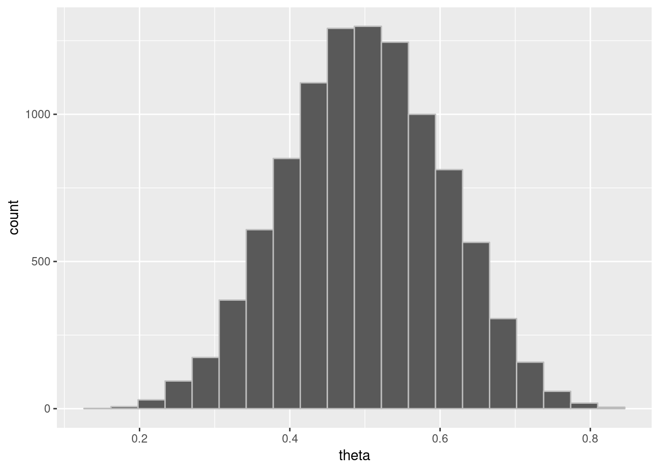
theta 0.32 0.00 0.10 0.20 0.45 3564 1
lp__ -14.29 0.01 0.76 -15.16 -13.77 4475 1
Samples were drawn using NUTS(diag_e) at Fri Jan 25 17:33:51 2019.
For each parameter, n_eff is a crude measure of effective sample size,
and Rhat is the potential scale reduction factor on split chains (at
convergence, Rhat=1).
- We obtain something similar to
Inference for Stan model: a6e9032b5e2c0ad2011961902392006a.
4 chains, each with iter=5000; warmup=2500; thin=1;
post-warmup draws per chain=2500, total post-warmup draws=10000.

        mean se_mean   sd    10%    90% n_eff Rhat
theta   0.23    0.00 0.09   0.12   0.34  3695    1
lp__  -12.30    0.01 0.71 -13.18 -11.80  3954    1

Samples were drawn using NUTS(diag_e)
For each parameter, n_eff is a crude measure of effective sample size,
and Rhat is the potential scale reduction factor on split chains (at
convergence, Rhat=1).
# Extracting the posterior draws

theta_draws = extract(fit)$theta

# Calculating posterior mean (estimator)
 mean(theta_draws)
[1] 0.3207932
# Calculating posterior intervals
 quantile(theta_draws, probs=c(0.10, 0.90))
      10%       90%
0.1968843 0.4486509
theta_draws_df = data.frame(list(theta = theta_draws))

plotpostre = ggplot(theta_draws_df, aes(x = theta)) +
geom_histogram(bins=20, color = "gray")
plotpostre
RStan: MAP, penalized MLE
Stan's optimization for estimation; two views:
- max posterior mode, also known as max a posteriori (MAP)
- max penalized likelihood (MLE)
library(rstan)
N = 5
y = c(0,1,1,0,0)

model = stan_model(model_code=bern.stan)

mle = optimizing(model, data=c("N", "y"))
print(mle, digits=2)
$par
theta
  0.4

$value
[1] -3.4

$return_code
[1] 0
Lotka-Volterra's (1927) Model
Lotka (1925) and Volterra (1926) formulated parametric differential equations that characterize the oscillating populations of predators and preys.
A statistical model to account for measurement error and unexplained variation uses the deterministic solutions to the Lotka-Volterra equations as expected population sizes.
Full Bayesian inference may be used to estimate future (or past) populations.
Stan is used to encode the statistical model and perform full Bayesian inference to solve the inverse problem of inferring parameters from noisy data.
In this example, we want to fit the model to Canadian lynx predator and snowshoe hare prey with repective populations between 1900 and 1920.
Notations and mathematical model
- \( u(t) \) prey,
- \( v(t) \) predator
\[ \frac{d}{dt}u = (\alpha -\beta v)u \]
\[ \frac{d}{dt}v=(-\gamma +\delta u)v \]
- \( \alpha \): prey growth, intrinsic
- \( \beta \): prey shrinkage due to predation
- \( \gamma \): predator shrinkage, intrinsic
- \( \delta \): predator growth from predation
Lotka-Volterra in Stan
real[] dz_dt(data real t,       // time
  real[] z,                     // system state
  real[] theta,                 // parameters
  data real[] x_r,              // real data
  data int[] x_i) {             // integer data

real u = z[1];                  // extract state
real v = z[2];
real alpha = theta[1];
real beta = theta[2];
real gamma = theta[3];
real delta = theta[4];

real du_dt = (alpha - beta * v) * u;
real dv_dt = (-gamma + delta * u) * v;
return { du_dt, dv_dt };
}
Known variables are observed
\( y_{n,k} \): denotes for species \( k \) at times \( t_{n} \) for \( n \in 0:N \)
Unknown variables must be inferred (inverse problem)
initial state: \( z_{k}^{init} \): initial population for \( k \)
subsequent states \( z_{n,k} \): population \( k \) at time \( t_{n} \)
parameters \( \alpha \), \( \beta \), \( \gamma \), \( \delta > 0 \)
Likelihood assumes errors are proportional (not additive)
\[ y_{n,k}\sim LogNormal(\hat{z}_{n,k}, \sigma_{k}), \]
equivalently: \[ \log y_{n,k} = \log \widehat{z}_{n,k} + \epsilon_{n,k} \] with \[ \epsilon_{n,k} \sim Normal(0, \sigma_{k}) \]
Lotka-Volterra in Stan (data, parameters)
- Variables for known constants, observed data
data {
int<lower = 0> N;       // num measurements
real ts[N];             // measurement times > 0
real y0[2];             // initial pelts
real<lower=0> y[N,2];   // subsequent pelts
}
- Variables for unknown parameters
parameters {
real<lower=0> theta[4];    // alpha, beta, gamma, delta
real<lower=0> z0[2];       // initial population
real<lower=0> sigma[2];    // scale of prediction error
}
Lotka-Volterra in Stan (priors, likelihood)
Sampling statements for priors and likelihood
model {
// priors
sigma ~ lognormal(0, 0.5);
theta[{1, 3}] ~ normal(1, 0.5);
theta[{2, 4}] ~ normal(0.05, 0.05);
z0[1] ~ lognormal(log(30), 5);
z0[2] ~ lognormal(log(5), 5);

// likelihood (lognormal)
for (k in 1:2) {
y0[k] ~ lognormal(log(z0[k]), sigma[k]);
y[ , k] ~ lognormal(log(z[, k]), sigma[k]);
}
}
Lotka-Volterra in Stan (solution to ODE)
We have to define variables for populations predicted by
ode, given:System function (
dz_dt), initial populations (z0).initial time (
0.0), solution times (ts).parameters (
theta), data arrays.tolerances (
1e-6, 1-e4), max iterations (1e3).
transformed parameters {
real z[N, 2]
= integrate_ode_rk45(dz_dt, z0, 0.0, ts, theta,
rep_array(0.0, 0), rep_array(0, 0),
1e-6, 1e-4, 1e3);
}
Lotka-Volterra Parameter Estimates
fit = stan(model_code=lotka-volterra.stan, data = lynx_hare_data)

print(fit, c("theta", "sigma"), probs=c(0.1, 0.5, 0.9))
            mean  se_mean   sd  10%  50%  90%  n_eff  Rhat
theta[1]    0.55    0     0.07 0.46 0.54 0.64   1168     1
theta[2]    0.03    0     0.00 0.02 0.03 0.03   1305     1
theta[3]    0.80    0     0.10 0.68 0.80 0.94   1117     1
theta[4]    0.02    0     0.00 0.02 0.02 0.03   1230     1
sigma[1]    0.29    0     0.05 0.23 0.28 0.36   2673     1
sigma[2]    0.29    0     0.06 0.23 0.29 0.37   2821     1
Obtained Results
Rhat near 1 signals convergence; n_eff is effective sample size
10%, … posterior quantiles; e.g., \( P[\alpha \in (0.46,0.64)|y]=0.8 \)
posterior mean is Bayesian point estimate: \( \alpha = 0.55 \)
standard error in posterior mean estimate is 0 (with rounding)
posterior standard deviation of \( \alpha \) estimated as 0.07
Other references and examples of Stan
- Andrew Gelman's blog about Rstan in RStudio Cloud
https://andrewgelman.com/2018/10/12/stan-on-the-web-for-free-thanks-to-rstudio
- Examples Session in RStudio Cloud
https://rstudio.cloud/project/56157
But I had problems to run these codes in the Cloud: RStudio in Cloud is version alpha :-(
Anyway, all examples of his blog can be donloaded from
https://github.com/stan-dev/example-models/archive/master.zip
Development Team of STAN
Andrew Gelman, Bob Carpenter, Daniel Lee, Ben Goodrich, Michael Betancourt, Marcus Brubaker, Jiqiang Guo, Allen Riddell, Marco Inacio, Jeffrey Arnold, Mitzi Morris, Rob Trangucci, Rob Goedman, Brian Lau, Jonah Sol Gabry, Robert L. Grant, Krzysztof Sakrejda, Aki Vehtari, Rayleigh Lei, Sebastian Weber, Charles Margossian, Vincent Picaud, Imad Ali, Sean Talts, Ben Bales, Ari Hartikainen, Matthijs Vakar, Andrew Johnson, Dan Simpson