The aim of this tutorial is to show the use of TensorFlow with KERAS for classification and prediction in Time Series Analysis. The latter just implement a Long Short Term Memory (LSTM) model (an instance of a Recurrent Neural Network which avoids the vanishing gradient problem).
Introduction
The code below has the aim to quick introduce Deep Learning analysis with TensorFlow using the Keras back-end in R environment. Keras is a high-level neural networks API, developed with a focus on enabling fast experimentation and not for final products. Keras and in particular the keras R package allows to perform computations using also the GPU if the installation environment allows for it.
Installing KERAS and TensorFlow in Windows … otherwise it will be more simple
- Install Anaconda: https://www.anaconda.com/download/
- Install Rtools(34): https://cran.r-project.org/bin/windows/Rtools/
GPU-TensorFlow
To use the option GPU-TensorFlow, you need CUDA Toolkit that matches the version of your GCC compiler: https://developer.nvidia.com/cuda-toolkit
If you have Python (i.e. Anaconda) just
install.packages("keras")
library(keras)
install_keras()
and this will install the Google Tensorflow module in Python.
If you want it working on GPU and you have a suitable CUDA version, you can install it with tensorflow = "gpu" option
install_keras(tensorflow = "gpu")
Simple check
library(keras)
to_categorical(0:3)
##      [,1] [,2] [,3] [,4]
## [1,]    1    0    0    0
## [2,]    0    1    0    0
## [3,]    0    0    1    0
## [4,]    0    0    0    1
Background on Neural Networks
Example old faithful IRIS data
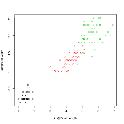
Consider the well-known IRIS data set
rm(list=ls())
data(iris)
plot(iris$Petal.Length,
 iris$Petal.Width, col = iris$Species)
head(iris)
##   Sepal.Length Sepal.Width Petal.Length Petal.Width Species
## 1          5.1         3.5          1.4         0.2  setosa
## 2          4.9         3.0          1.4         0.2  setosa
## 3          4.7         3.2          1.3         0.2  setosa
## 4          4.6         3.1          1.5         0.2  setosa
## 5          5.0         3.6          1.4         0.2  setosa
## 6          5.4         3.9          1.7         0.4  setosa
We want to build an iris specie classifier based on the observed four iris dimensions. This is the usual classification (prediction) problem so we have to consider a training sample and evaluate the classifier on a test sample.
Data in TensorFlow
Data are
- Matrices ```matrix´´´ of doubles.
- Categorical variables need to be codified in dummies: one hot encoding.
onehot.species = to_categorical(as.numeric(iris$Species) - 1)
iris = as.matrix(iris[, 1:4])
iris = cbind(iris, onehot.species)
Training and Test Data Sets
Define training and test
set.seed(17)
ind <- sample(2, nrow(iris),
replace = TRUE, prob = c(0.7, 0.3))
iris.training <- iris[ind == 1, 1:4]
iris.test <- iris[ind == 2, 1:4]
iris.trainingtarget <- iris[ind == 1, -seq(4)]
iris.testtarget <- iris[ind == 2, -(1:4)]
Model building
Initialize the model
model <- keras_model_sequential()
and suppose to use a very simple one
model %>%
 layer_dense(units = ncol(iris.trainingtarget), activation = 'softmax',
 input_shape = ncol(iris.training))
summary(model)
## ___________________________________________________________________________
## Layer (type)                     Output Shape                  Param #
## ===========================================================================
## dense_1 (Dense)                  (None, 3)                     15
## ===========================================================================
## Total params: 15
## Trainable params: 15
## Non-trainable params: 0
## ___________________________________________________________________________
This is the model structure:
model$inputs
## [[1]]
## Tensor("dense_1_input:0", shape=(?, 4), dtype=float32)
model$outputs
## [[1]]
## Tensor("dense_1/Softmax:0", shape=(?, 3), dtype=float32)
and a graphical representation:
library(igraph)
##
## Attaching package: 'igraph'
## The following objects are masked from 'package:keras':
##
##     %<-%, normalize
## The following objects are masked from 'package:stats':
##
##     decompose, spectrum
## The following object is masked from 'package:base':
##
##     union
g = graph_from_literal(Sepal.Length:Sepal.Width:Petal.Length:Petal.Width---Species,simplify = TRUE)
layout <- layout_in_circle(g, order = order(degree(g)))
plot(g,layout = layout,vertex.color = c(2,2,2,2,3))
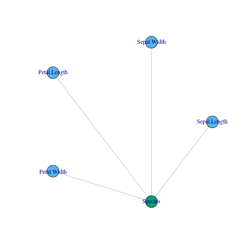
In the plot, blue colors stand for input and green ones for output.
Its analytic representation is the following one:
$$Species_j = act.func(\mathbf{w}_j,\mathbf{x} = (PW,PL,SW,SL)),$$
where the activation function is the softmax (the all life logistic!):
$$act.func(\mathbf{w}_j,\mathbf{x}) = \frac{e^{\mathbf{x}^T\mathbf{w}}}{\sum e^{\mathbf{x}^T\mathbf{w}}}$$
which estimates $Pr(Specie = j|\mathbf{x} = (PW,PL,SW,SL))$.
Model fitting: fit() and the optimizer
Estimation consists in finding the weights $\mathbf{w}$ that minimizes a loss function. For instance, if the response $Y$ were quantitative, then
$$w = \arg\min \sum_{i = 1}^m(y_i-wx_i)^2,$$
whose solution is given by the usual equations of derivatives $w$:
$$\frac{\partial \sum_{i = 1}^n(y_i-wx_i)^2}{\partial w} = 0,$$
Note however, that
$$\partial \sum (y_i-wx_i)^2 = \sum \partial (y_i-wx_i)^2,$$
(Is parallelizable in batches of samples (of length batch_size), that is
$$\sum \partial (y_i-wx_i)^2 = \sum{\partial\sum (y_i-wx_i)^2}$$
where $n_l$ is the batch_size.
Suppose in general a non-analytical loss function (the usual case in more complicated networks) $Q(w) = \sum_{i = 1}^m(y_i-wx_i)^2,$ and suppose that $\frac{\partial Q(w)}{\partial w} = 0$ is not available analytically. Then we would have to use “Newton-Raphson” optimizer family (or gradient optimizers) whose best known member in Deep Learning (DL) is the Stochastic Gradient Descent (SGD):
Starting form an initial weight $w^{(0)}$ at step $m$:
$$w^{(m)} = w^{(m-1)}-\eta\Delta Q_i(w),$$ where $\eta>0$ is the Learning Rate: the lower (bigger) $\eta$ is, the more (less) steps are needed to achieve the optimum with a greater (worse) precision.
It is stochastic in the sense that the index $i$ of the sample is random (avoids overfitting): $\Delta Q(w) : = \Delta Q_i(w)$. This also induces complications when (if) dealing with time series.
There are other variations to the SGD: Momentum, Averaging, AdaGrad, Adam, …
Using SGD with $\eta = 0.01$ we have to set:
sgd <- optimizer_sgd(lr = 0.01)
and then this is plugged in into the model and used afterwards in compilation. Once it is established, the loss function $Q$ (here we use the categorical_crossentropy because the response is a non-binary categorical variable):
model %>% compile(
 loss = 'categorical_crossentropy',
 optimizer = sgd,
 metrics = 'accuracy'
)
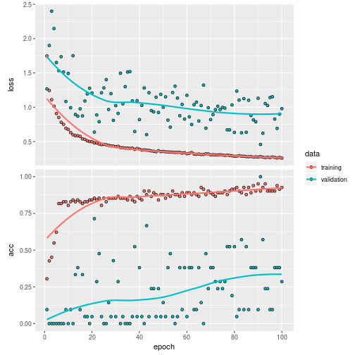
we have to train it in epochs (i.e. the $m$ steps above) using a portion of the training sample, validation_split, to verify eventual overfitting (i.e. the model is fitted and the loss evaluated in that random part of the sample which is finally not used for training):
history <- model %>% fit(
 x = iris.training,
 y = iris.trainingtarget,
 epochs = 100,
 batch_size = 5,
 validation_split = 0.2,
 verbose = 0
)
The result of the trained model is:
plot(history)
Validation on the test sample:
classes <- model %>% predict_classes(iris.test)
table(iris.testtarget%*%0:2, classes)
##    classes
##      0  1  2
##   0 20  0  0
##   1  0 12  0
##   2  0  7  8
with a validation score
(score <- model %>% evaluate(iris.test, iris.testtarget))
## $loss
## [1] 0.3292574
##
## $acc
## [1] 0.8510638
Another example: Classification of breast cancer
We have 10 variables (all factors) and a binary response: benign versus malign.
library(mlbench)
data(BreastCancer)
dim(BreastCancer)
## [1] 699 11
levels(BreastCancer$Class)
## [1] "benign" "malignant"
head(BreastCancer)
##        Id Cl.thickness Cell.size Cell.shape Marg.adhesion Epith.c.size
## 1 1000025            5         1          1             1            2
## 2 1002945            5         4          4             5            7
## 3 1015425            3         1          1             1            2
## 4 1016277            6         8          8             1            3
## 5 1017023            4         1          1             3            2
## 6 1017122            8        10         10             8            7
##   Bare.nuclei Bl.cromatin Normal.nucleoli Mitoses     Class
## 1           1           3               1       1    benign
## 2          10           3               2       1    benign
## 3           2           3               1       1    benign
## 4           4           3               7       1    benign
## 5           1           3               1       1    benign
## 6          10           9               7       1 malignant
str(BreastCancer)
## 'data.frame':	699 obs. of  11 variables:
##  $ Id             : chr  "1000025" "1002945" "1015425" "1016277" ...
##  $ Cl.thickness   : Ord.factor w/ 10 levels "1"<"2"<"3"<"4"<..: 5 5 3 6 4 8 1 2 2 4 ...
##  $ Cell.size      : Ord.factor w/ 10 levels "1"<"2"<"3"<"4"<..: 1 4 1 8 1 10 1 1 1 2 ...
##  $ Cell.shape     : Ord.factor w/ 10 levels "1"<"2"<"3"<"4"<..: 1 4 1 8 1 10 1 2 1 1 ...
##  $ Marg.adhesion  : Ord.factor w/ 10 levels "1"<"2"<"3"<"4"<..: 1 5 1 1 3 8 1 1 1 1 ...
##  $ Epith.c.size   : Ord.factor w/ 10 levels "1"<"2"<"3"<"4"<..: 2 7 2 3 2 7 2 2 2 2 ...
##  $ Bare.nuclei    : Factor w/ 10 levels "1","2","3","4",..: 1 10 2 4 1 10 10 1 1 1 ...
##  $ Bl.cromatin    : Factor w/ 10 levels "1","2","3","4",..: 3 3 3 3 3 9 3 3 1 2 ...
##  $ Normal.nucleoli: Factor w/ 10 levels "1","2","3","4",..: 1 2 1 7 1 7 1 1 1 1 ...
##  $ Mitoses        : Factor w/ 9 levels "1","2","3","4",..: 1 1 1 1 1 1 1 1 5 1 ...
##  $ Class          : Factor w/ 2 levels "benign","malignant": 1 1 1 1 1 2 1 1 1 1 ...
Data in matrices
tt = BreastCancer[complete.cases(BreastCancer),2:11]
x = NULL
for(i in seq(9)) x = cbind(x,to_categorical(as.numeric(tt[,i])-1))
y = to_categorical(as.numeric(tt[,10])-1)
head(y)
##      [,1] [,2]
## [1,]    1    0
## [2,]    1    0
## [3,]    1    0
## [4,]    1    0
## [5,]    1    0
## [6,]    0    1
Set training and test
set.seed(17)
ind <- sample(2, nrow(x),
 replace = TRUE, prob = c(0.7, 0.3))

x.train = x[ind == 1,]
y.train = y[ind == 1,]
x.test = x[ind == 2,]
y.test = y[ind == 2,]
Let’s build the DL model with tree layers of neurons:
# Initialize a sequential model
model <- keras_model_sequential()

# Add layers to model
model %>%
 layer_dense(units = 8, activation = 'relu', input_shape = ncol(x.train)) %>%
 layer_dense(units = 5, activation = 'relu') %>%
 layer_dense(units = ncol(y.train), activation = 'softmax')

summary(model)
## ___________________________________________________________________________
## Layer (type)                     Output Shape                  Param #
## ===========================================================================
## dense_2 (Dense)                  (None, 8)                     720
## ___________________________________________________________________________
## dense_3 (Dense)                  (None, 5)                     45
## ___________________________________________________________________________
## dense_4 (Dense)                  (None, 2)                     12
## ===========================================================================
## Total params: 777
## Trainable params: 777
## Non-trainable params: 0
## ___________________________________________________________________________
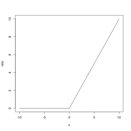
As activation function (being the response binary) we use a user defined relu ($f(x) = x^+$):
Let’s use the adam optimizer
# Compile the model
model %>% compile(
 loss = 'categorical_crossentropy',
 optimizer = "adam",
 metrics = 'accuracy'
)
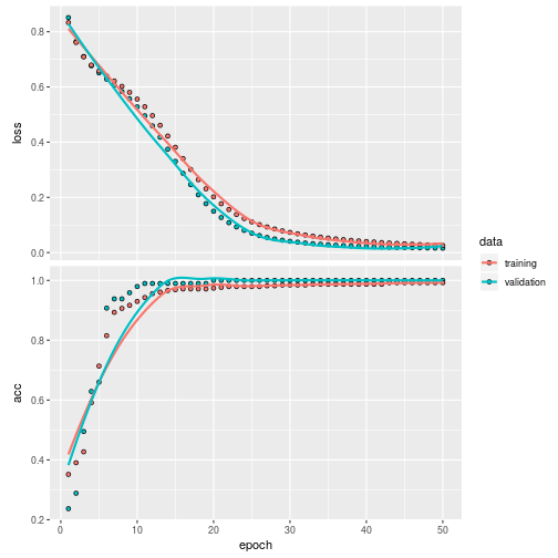
Train the model
history <- model %>% fit(
 x = x.train,
 y = y.train,
 epochs = 50,
 batch_size = 50,
 validation_split = 0.2,
 verbose = 2
)
plot(history)
Validate it on the test set
classes <- model %>% predict_classes(x.test)
table(y.test%*%0:1, classes)
##    classes
##       0   1
##   0 121   6
##   1   5  70
also with a score
(score <- model %>% evaluate(x.test, y.test))
## $loss
## [1] 0.1734528
##
## $acc
## [1] 0.9455446
LSTM model
Here we apply the DL to time series analysis: it is not possible to draw train and test randomly and they must be random sequences of train and test of length batch_size.
Data
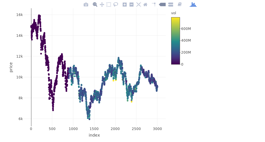
From Yahoo Finance let’s download the IBEX 35 time series on the last 15 years and consider the last 3000 days of trading:
library(BatchGetSymbols)
tickers <- c('%5EIBEX')
first.date <- Sys.Date() - 360*15
last.date <- Sys.Date()
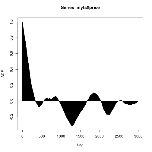
YAHOO database query and the ACF of the considered IBEX 35 series is here:
myts <- BatchGetSymbols(tickers = tickers,
 first.date = first.date,
 last.date = last.date,
 cache.folder = file.path(tempdir(),
 'BGS_Cache') ) # cache in tempdir()
##
## Running BatchGetSymbols for:
##    tickers = %5EIBEX
##    Downloading data for benchmark ticker | Not Cached
## %5EIBEX | yahoo (1|1) | Not Cached - Feliz que nem lambari de sanga!
print(myts$df.control)
##    ticker   src download.status total.obs perc.benchmark.dates
## 1 %5EIBEX yahoo              OK      3787            0.9903304
##   threshold.decision
## 1               KEEP
y = myts$df.tickers$price.close
myts = data.frame(index = myts$df.tickers$ref.date, price = y, vol = myts$df.tickers$volume)
myts = myts[complete.cases(myts), ]
myts = myts[-seq(nrow(myts) - 3000), ]
myts$index = seq(nrow(myts))

library(plotly)

plot_ly(myts, x = ~index, y = ~price, type = "scatter", mode = "markers", color = ~vol)
acf(myts$price, lag.max = 3000)
Training and Testing samples
Data must be standardized
msd.price = c(mean(myts$price), sd(myts$price))
msd.vol = c(mean(myts$vol), sd(myts$vol))
myts$price = (myts$price - msd.price[1])/msd.price[2]
myts$vol = (myts$vol - msd.vol[1])/msd.vol[2]
summary(myts)
##      index            price               vol
##  Min.   :   1.0   Min.   :-2.20595   Min.   :-1.2713
##  1st Qu.: 750.8   1st Qu.:-0.73810   1st Qu.:-1.2689
##  Median :1500.5   Median :-0.06936   Median : 0.1166
##  Mean   :1500.5   Mean   : 0.00000   Mean   : 0.0000
##  3rd Qu.:2250.2   3rd Qu.: 0.36329   3rd Qu.: 0.6992
##  Max.   :3000.0   Max.   : 3.00692   Max.   : 4.7057
Let’s use the first 2000 days for training and the last 1000 for test. Remember that the ratio between the number of train samples and test samples must be an integer number as also the ratio between these two lengths with batch_size. This is why 2000⁄1000, 2000⁄50 and 1000⁄50:
datalags = 10
train = myts[seq(2000 + datalags), ]
test = myts[2000 + datalags + seq(1000 + datalags), ]
batch.size = 50
Data for LSTM
Predictor $X$ is a 3D matrix: 1. first dimension is the length of the time series 2. second is the lag; 3. third is the number of variables used for prediction $X$ (at least 1 for the series at a given lag).
Response $Y$ is a 2D matrix: 1. first dimension is the length of the time series 2. second is the lag;
x.train = array(data = lag(cbind(train$price, train$vol), datalags)[-(1:datalags), ], dim = c(nrow(train) - datalags, datalags, 2))
y.train = array(data = train$price[-(1:datalags)], dim = c(nrow(train)-datalags, 1))

x.test = array(data = lag(cbind(test$vol, test$price), datalags)[-(1:datalags), ], dim = c(nrow(test) - datalags, datalags, 2))
y.test = array(data = test$price[-(1:datalags)], dim = c(nrow(test) - datalags, 1))
The LSTM model codified with Keras
model <- keras_model_sequential()

model %>%
 layer_lstm(units = 100,
 input_shape = c(datalags, 2),
 batch_size = batch.size,
 return_sequences = TRUE,
 stateful = TRUE) %>%
 layer_dropout(rate = 0.5) %>%
 layer_lstm(units = 50,
 return_sequences = FALSE,
 stateful = TRUE) %>%
 layer_dropout(rate = 0.5) %>%
 layer_dense(units = 1)

model %>%
 compile(loss = 'mae', optimizer = 'adam')

model
## Model
## ___________________________________________________________________________
## Layer (type)                     Output Shape                  Param #
## ===========================================================================
## lstm_1 (LSTM)                    (50, 10, 100)                 41200
## ___________________________________________________________________________
## dropout_1 (Dropout)              (50, 10, 100)                 0
## ___________________________________________________________________________
## lstm_2 (LSTM)                    (50, 50)                      30200
## ___________________________________________________________________________
## dropout_2 (Dropout)              (50, 50)                      0
## ___________________________________________________________________________
## dense_5 (Dense)                  (50, 1)                       51
## ===========================================================================
## Total params: 71,451
## Trainable params: 71,451
## Non-trainable params: 0
## ___________________________________________________________________________
Let’s train in 2000 steps. Remember: for being the model stateful (stateful = TRUE), which means that the signal state (the latent part of the model) is trained on the batch of the time series, you need to manually reset the states (batches are supposed to be independent sequences (!) ):
for(i in 1:2000){
 model %>% fit(x = x.train,
 y = y.train,
 batch_size = batch.size,
 epochs = 1,
 verbose = 0,
 shuffle = FALSE)
 model %>% reset_states()
}
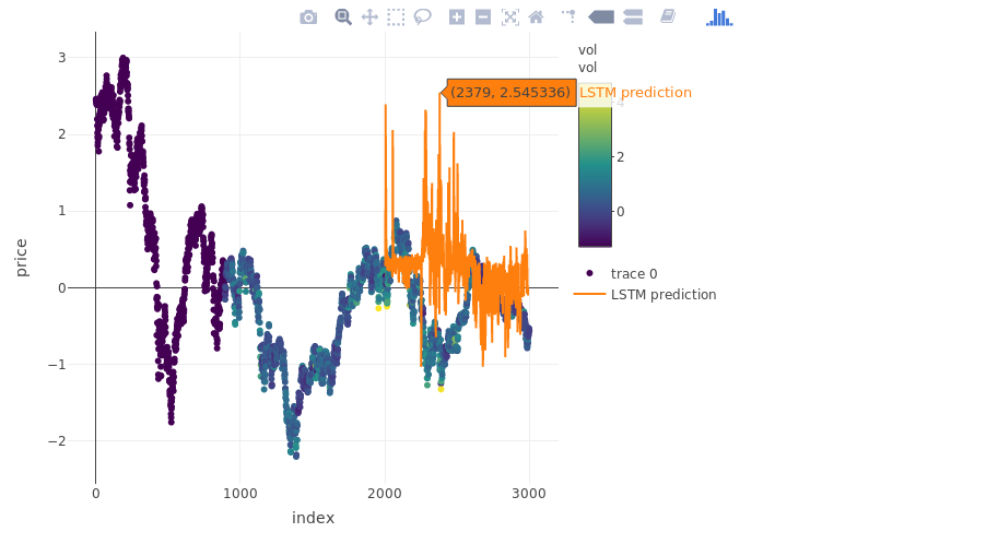
The prediction
pred_out <- model %>% predict(x.test, batch_size = batch.size) %>% .[,1]

plot_ly(myts, x = ~index, y = ~price, type = "scatter", mode = "markers", color = ~vol) %>%
 add_trace(y = c(rep(NA, 2000), pred_out), x = myts$index, name = "LSTM prediction", mode = "lines")
## Warning: line.color doesn't (yet) support data arrays
## Warning: line.color doesn't (yet) support data arrays
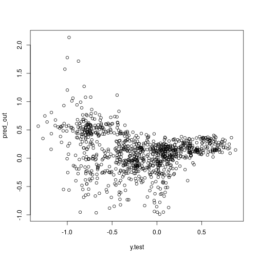
more on validation:
plot(x = y.test, y = pred_out)
Some notes on Deep Learning
A deep learning (DL) model is a neural network with many layers of neurons (Schmidhuber 2015), it is an algorithmic approach rather than probabilistic in its nature, see (Breiman and others 2001) for the merits of both approaches. Each neuron is a deterministic function such that a neuron of a neuron is a function of a function along with an associated weight $w$. Essentially for a response variable $Y_i$ for the unit $i$ and a predictor $X_i$ we have to estimate $Y_i = w_1f_1(w_2f_2(…(w_kf_k(X_i))))$, and the larger $k$ is, the “deeper” is the network. With many stacked layers of neurons all connected (a.k.a. dense layers) it is possible to capture high non-linearities and all interactions among variables. The approach to model estimation underpinned by a DL model is that of composition function against that od additive function underpinned by the usual regression techniques including the most modern one (i.e. $Y_i = w_1f_1(X_i)+w_2f_2(X_i)+…+w_kf_k(X_i)$). A thorough review of DL can be found at (Schmidhuber 2015).
Likely the DL model can be also interpreted as a maximum a posteriori estimation of $Pr(Y|X,Data)$ (Polson, Sokolov, and others 2017) for Gaussian process priors. Despite this and because of its complexity it cannot be evaluated the whole distribution $Pr(Y|X,Data)$, but only its mode.
Estimating a DL consists in just estimating the vectors $w_1,\ldots,w_k$. The estimation requires to evaluate a multidimensional gradient which is not possible to be evaluated jointly for all observations, because of its dimensionality and complexity. Recalling that the derivative of a composite function is defined as the product of the derivative of inner functions (i.e. the chain rule $(f\circ g)’ = (f’\circ g)\cdot g’$) which is implemented for purposes of computational feasibility as a tensor product. Such tensor product is evaluated for batches of observations and it is implemented in the open source software known as Google Tensor Flow (Abadi et al. 2015).
Fundamentals of LSTM can be found here (Sherstinsky 2018) (it needs some translation to the statistical formalism).
References
Abadi, Martín, Ashish Agarwal, Paul Barham, Eugene Brevdo, Zhifeng Chen, Craig Citro, Greg S. Corrado, et al. 2015. “TensorFlow: Large-Scale Machine Learning on Heterogeneous Systems.” URL: https://www.tensorflow.org/.
Breiman, Leo, and others. 2001. “Statistical Modeling: The Two Cultures (with Comments and a Rejoinder by the Author).” Statistical Science 16 (3). Institute of Mathematical Statistics: 199-231.
Polson, Nicholas G, Vadim Sokolov, and others. 2017. “Deep Learning: A Bayesian Perspective.” Bayesian Analysis 12 (4). International Society for Bayesian Analysis: 1275-1304.
Schmidhuber, Jürgen. 2015. “Deep Learning in Neural Networks: An Overview.” Neural Networks 61. Elsevier: 85-117.
Sherstinsky, Alex. 2018. “Fundamentals of Recurrent Neural Network (Rnn) and Long Short-Term Memory (Lstm) Network,” August. URL: http://arxiv.org/abs/http://arxiv.org/abs/1808.03314v4.