Introduction
In this session I will focus on Bayesian inference using the integrated nested
Laplace approximation (INLA) method. As described in Rue et al. (2009), INLA
can be used to estimate the posterior marginal distribution of Bayesian
hierarchical models. This method is implemented in the INLA package available
for the R programming language. Given that the types of models that INLA can
fit are quite wide, we will focus on spatial models for the analysis of lattice
data. Hence,
Bayesian inference
A Bayesian hierarchical model can be defined as follows:
\[ y_i \sim f(y_i \mid \mathbf{x}, \theta_1) \]
\[ \mathbf{x} \sim GMRF(\theta_2) \]
\[ \theta \sim \pi(\theta) \]
Here, \(\mathbf{y} = (y_1, \ldots, y_n)\) is a vector of responses, \(\mathbf{x}\) a vector of latent effects and \(\theta = (\theta_1, \theta_2)\) a vector of hyperparameters. \(GMRF(\theta_2)\) is a Gaussian Markov random field (GMRF) with zero mean, which can be regarded as a multivariate Gaussian distribution with zero mean and sparse precision matrix that depends on hyperparameters \(\theta_2\).
Fitting a Bayesian model means computing the posterior distribution of \(\mathbf{x}\) and \(\theta\) \(\pi(\theta, \mathbf{x} \mid y)\). This can be obtained by using Bayes’ rule as follows:
\[ \pi(\theta, \mathbf{x} \mid y) \propto \pi(y \mid \theta, \mathbf{x})\pi(\theta) \]
Once the joint posterior distribution is known, we could compute posterior probabilities of linear predictors, random effects, sums of random effects, etc. Depending on the likelihood and the prior distribution computing \(\pi(\theta, \mathbf{x} \mid y)\) can be very difficult.
Inference with Markov chain Monte Carlo
In the last 20-30 years some computational approaches have been proposed to estimate \(\pi(\theta, \mathbf{x} \mid y)\) with Monte Carlo methods. In particular, Markov chain Monte Carlo (MCMC) methods provide simulations from the ensemble of model parameters, i.e., a multivariate distribution. This will allow us to estimate the joint posterior distribution.
However, we may be interested in a single parameter or a subset of the parameters. Inference for this subset of parameters can be done by simply ignoring the samples for the other parameters
Using the samples it is possible to compute the posterior distribution of any function on the model parameters. Notice that MCMC may require lots of simulations for valid inference. Also, we must check that the burn-in period has ended, i.e., we have reached the posterior distribution
Integrated Nested Laplace Approximation
Sometimes we only need marginal inference on some parameters, i.e., we need \(\pi(\theta_i \mid y)\). Rue et al. (2009) propose a way of approximating the marginal distributions using different approximations to the distributions involved and using the Laplace approximation for the integrals.
Now we are dealing with (many) univariate distributions. This is computationally faster because numerical integration techniques are used instead of Monte Carlo sampling. The marginal distributions for the latent effects and hyper-parameters can be written as
\[ \pi(x_i \mid \mathbf{y}) = \int \pi(x_i \mid \mathbf{\theta}, \mathbf{y}) \pi(\mathbf{\theta}\mid \mathbf{y}) d\mathbf{\theta} \] and
\[ \pi(\theta_j\mid \mathbf{y}) = \int \pi(\mathbf{\theta}\mid \mathbf{y}) d\mathbf{\theta}_{-j} \]
The posterior distribution of the hyperparameters \(\pi(\mathbf{\theta}\mid \mathbf{y})\) is approximated using different methods.
R-INLA package
The INLA method is implemented in the INLA (also known as R-INLA) package,
which is available from http://www.r-inla.org.
This package relies on the inla()-function to fit the models. This functions
works in a similar way as, for example, glm(). The model is defined in a and there is a flexible way of defining the likelihood, priors and
latent effects in the model.
The output provides the posterior marginals of the model parameters and latent
effects, linear predictors, and some other derived quantities (such as linear
combinations of the model latent effects). In addition, INLA provides tools
to manipulate \(\pi(\cdot \mid y)\) to compute \(\pi(f(\cdot) \mid y)\). INLA can compute some model assessment/choice: Marginal likelihood, DIC, CPO, …
Spatial latent effects
The following table summarizes some of the spatial latent effects available
in INLA:
Name in f() |
Model |
|---|---|
generic0 |
\(\Sigma=\frac{1}{\tau}Q^{-1}\) |
generic1 |
\(\Sigma=\frac{1}{\tau}(I_n-\frac{\rho}{\lambda_{max}}C)^{-1}\) |
besag |
Intrinsic CAR |
besagproper |
Proper CAR |
bym |
Convolution model |
rw2d |
Random walk 2-D |
matern2d |
Matèrn correlation (discrete) |
slm |
Spatial lag model |
spde |
Matèrn correlation (continuous) |
Dataset: Leukemia in upstate New York
To illustrate how spatial models are fitted with INLA, the New York leukemia
dataset will be used. This has been widely analyzed in the literature (see, for
example, Waller and Gotway, 2004) and it is available in the DClusterm
package. The dataset records a number of cases of leukemia in upstate New York
at the census tract level. Some of the variables in the dataset are:
Cases: Number of leukemia cases in the period 1978-1982.POP8: Population in 1980.PCTOWNHOME: Proportion of people who own their home.PCTAGE65P: Proportion of people aged 65 or more.AVGIDIST: Average inverse distance to the nearest Trichloroethene (TCE) site.
Note that the interest is on the exposure to TCE, using AVGIDIST as a proxy
for exposure. Variables PCTOWNHOME and PCTAGE65P will act as possible
confounders that must be included in the model. However, we will not do it
here because we want to test how the spatial latent effects capture residual
spatial variation.
The dataset can be loaded as follows:
library(spdep)
library(DClusterm)
data(NY8)
Given that the interest is in studying the risk of leukemia in upstate New York, the expected number of cases is computed first. This is done by computing the overall mortality rate (total cases divided by total population) and multiplying the population by it:
rate <- sum(NY8$Cases) / sum(NY8$POP8)
NY8$Expected <- NY8$POP8 * rate
Once the expected number of cases is obtained, a raw estimate of risk can be obtained with the standardized mortality ratio (SMR), which is computed as the number of observed cases divided by the number of expected cases:
NY8$SMR <- NY8$Cases / NY8$ExpectedDisease mapping
In Epidemiology it is important to produce maps to show the spatial distribution of the relative risk. In this example, we will focus on Syracuse city to reduce the computation time to produce the map. Hence, we create an index with the areas in Syracuse city:
# Subset Syracuse city
syracuse <- which(NY8$AREANAME == "Syracuse city")
A disease map can be simply created with function spplot (in package
sp):
library(viridis)## Loading required package: viridisLitespplot(NY8[syracuse, ], "SMR", #at = c(0.6, 0.9801, 1.055, 1.087, 1.125, 13),
col.regions = rev(magma(16))) #gray.colors(16, 0.9, 0.4))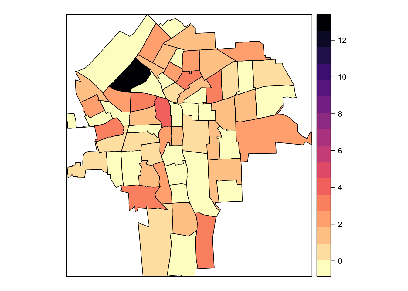
Interactive maps can be easily created with the tmap package:
library(tmap)
tmap_mode("view")

SMR_map <- tm_shape(NY8[syracuse, ]) +
  tm_fill(col = "SMR", alpha = 0.35) +
  tm_borders() +
  tm_shape(TCE) + tm_dots(col = "red") # Add TCE sites
widgetframe::frameWidget(print(SMR_map))
Note that the previous map also includes the locations of the 11 TCE-contaminated sites and that this can be seen by zooming out.
Mixed-effects models
Poisson regression
The first model that we will consider is a Poisson model with no latent random effects as this will provide a baseline to compare to other models. The model to fit is:
\[ O_i|\mu_i \sim Po(\mu_i) \]
\[ \mu_i = E_i \theta_i \]
\[ \log(\theta_i) = \beta_0 + \beta_1 AVGIDIST_i \]
In order to fit the model with INLA, function inla is used:
library(INLA)
m1 <- inla(Cases ~ 1 + AVGIDIST,
   data = as.data.frame(NY8),
  family = "poisson",
  E = NY8$Expected, control.predictor = list(compute = TRUE),
  control.compute = list(dic = TRUE, waic = TRUE))
Note that it works similarly to the glm function. Here, argument
E is used for the expected number of cases. Alternatively, they could
enter the linear predictor in the log-scale as an offset.
Other arguments are set to compute the marginals of the model parameters
(with control.predictor) and to compute some model choice criteria
(with control.compute).
Next, the summary of the model can be obtained:
summary(m1)##
## Call:
## c("inla(formula = Cases ~ 1 + AVGIDIST, family = \"poisson\", data
## = as.data.frame(NY8), ", " E = NY8$Expected, control.compute =
## list(dic = TRUE, waic = TRUE), ", " control.predictor =
## list(compute = TRUE))")
## Time used:
## Pre = 0.368, Running = 0.0968, Post = 0.0587, Total = 0.524
## Fixed effects:
## mean sd 0.025quant 0.5quant 0.975quant mode kld
## (Intercept) -0.065 0.045 -0.155 -0.065 0.023 -0.064 0
## AVGIDIST 0.320 0.078 0.160 0.322 0.465 0.327 0
##
## Expected number of effective parameters(stdev): 2.00(0.00)
## Number of equivalent replicates : 140.25
##
## Deviance Information Criterion (DIC) ...............: 948.12
## Deviance Information Criterion (DIC, saturated) ....: 418.75
## Effective number of parameters .....................: 2.00
##
## Watanabe-Akaike information criterion (WAIC) ...: 949.03
## Effective number of parameters .................: 2.67
##
## Marginal log-Likelihood: -480.28
## Posterior marginals for the linear predictor and
## the fitted values are computedPoisson regression with random effects
Latent random effects can be added to the model to account for overdispersion by including i.i.d. Gaussian random effects in the linear predictor, as follows:
\[ O_i|\mu_i \sim Po(\mu_i) \]
\[ \mu_i = E_i \theta_i \]
\[ \log(\theta_i) = \beta_0 + \beta_1 AVGIDIST_i + u_i \]
\[ u_i \sim N(0, \tau) \]
In order to fit the model with INLA an index to identify
the random effects (ID) is created first. Latent random effects
are specified with the f-function in INLA:
NY8$ID <- 1:nrow(NY8)
m2 <- inla(Cases ~ 1 + AVGIDIST + f(ID, model = "iid"),
  data = as.data.frame(NY8), family = "poisson",
  E = NY8$Expected,
  control.predictor = list(compute = TRUE),
  control.compute = list(dic = TRUE, waic = TRUE))
Now the summary of the mode includes information about the random effects:
summary(m2)##
## Call:
## c("inla(formula = Cases ~ 1 + AVGIDIST + f(ID, model = \"iid\"),
## family = \"poisson\", ", " data = as.data.frame(NY8), E =
## NY8$Expected, control.compute = list(dic = TRUE, ", " waic =
## TRUE), control.predictor = list(compute = TRUE))" )
## Time used:
## Pre = 0.236, Running = 0.315, Post = 0.0744, Total = 0.625
## Fixed effects:
## mean sd 0.025quant 0.5quant 0.975quant mode kld
## (Intercept) -0.126 0.064 -0.256 -0.125 -0.006 -0.122 0
## AVGIDIST 0.347 0.105 0.139 0.346 0.558 0.344 0
##
## Random effects:
## Name Model
## ID IID model
##
## Model hyperparameters:
## mean sd 0.025quant 0.5quant 0.975quant mode
## Precision for ID 3712.34 11263.70 3.52 6.94 39903.61 5.18
##
## Expected number of effective parameters(stdev): 54.95(30.20)
## Number of equivalent replicates : 5.11
##
## Deviance Information Criterion (DIC) ...............: 926.93
## Deviance Information Criterion (DIC, saturated) ....: 397.56
## Effective number of parameters .....................: 61.52
##
## Watanabe-Akaike information criterion (WAIC) ...: 932.63
## Effective number of parameters .................: 57.92
##
## Marginal log-Likelihood: -478.93
## Posterior marginals for the linear predictor and
## the fitted values are computedAdd point estimates for mapping
The posterior means estimated with these two models can be added to
the SpatialPolygonsDataFrame NY8 to be plotted later:
NY8$FIXED.EFF <- m1$summary.fitted[, "mean"]
NY8$IID.EFF <- m2$summary.fitted[, "mean"]
spplot(NY8[syracuse, ], c("SMR", "FIXED.EFF", "IID.EFF"),
col.regions = rev(magma(16)))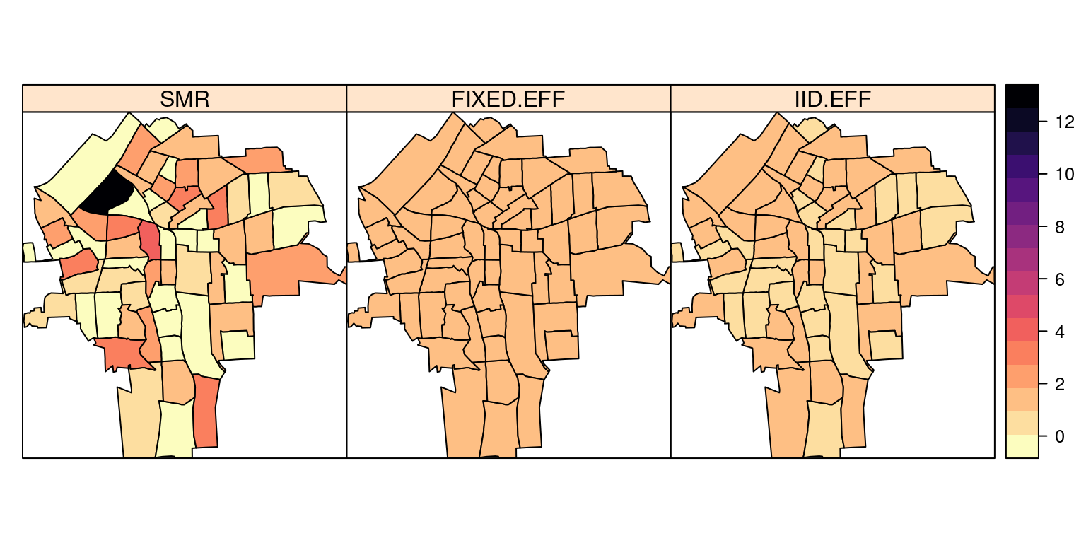
Note how the model smooths the relative risk.
Spatial Models for Lattice Data
Lattice data involves data measured at different areas, e.g., neighborhoods, cities, provinces, states, etc. Spatial dependence appears because neighbor areas will show similar values of the variable of interest.
Models for lattice data
We have observations \(y=\{y_i\}_{i=1}^n\) from the \(n\) areas. \(\mathbf{y}\) is assigned a multivariate distribution that accounts for spatial dependence. A common way of describing spatial proximity in lattice data is by means of an adjacency matrix \(W\). Element \(W_{i, j}\) is non-zero if areas \(i\) and \(j\) are neighbors. Usually, two areas are neighbors if they share a common boundary. There are other definitions of neighborhood (see Bivand et al., 2013).
Adjacency matrix
The adjacency matrix can be computed using function poly2nb in package
spdep. This function will consider two areas as neighbors if their borders
touch at least in one point (i.e., queen adjacency):
NY8.nb <- poly2nb(NY8)This will return an nb object with the definition of the neighborhood structure:
NY8.nb## Neighbour list object:
## Number of regions: 281
## Number of nonzero links: 1624
## Percentage nonzero weights: 2.056712
## Average number of links: 5.779359In addition, nb objects can be plot when the centroids of the polygons are
known:
plot(NY8)
plot(NY8.nb, coordinates(NY8), add = TRUE, pch = ".", col = "gray")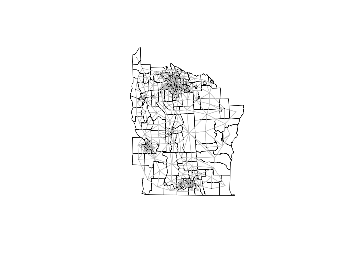
Regression models
It is often the case that, in addition to \(y_i\), we have a number of covariates \(X_i\). Hence, we may want to regress \(y_i\) on \(X_i\). In addition to the covariates we may want to account for the spatial structure of the data. Different types of regression models can be used to model lattice data:
- Generalized Linear Models (with spatial random effects).
- Spatial econometrics models.
Linear Mixed Models
A common approach (for Gaussian data) is to use a linear regression with random effects:
\[ Y = X \beta+ Zu +\varepsilon \]
The vector of random effects \(u\) is modeled as a multivariate Normal distribution:
\[ u \sim N(0, \sigma^2_u \Sigma) \]
\(\Sigma\) is defined such as it induces higher correlation with adjacent areas, \(Z\) is a design matrix for the random effects and \(\varepsilon_i \sim N(0, \sigma^2), i=1, \ldots, n\) is an error term.
Generalized Linear Mixed Models can be defined in a similar way by using a different likelihood and linking the appropriate parameter to the linear predictor.
Structure of spatial random effects
There are many different ways of including spatial dependence in \(\Sigma\):
- Simultaneous autoregressive (SAR):
\[ \Sigma^{-1} = [(I-\rho W)' (I-\rho W)] \]
- Conditional autoregressive (CAR):
\[ \Sigma^{-1} = (I-\rho W) \]
Intrinsic CAR (ICAR):
\[ \Sigma^{-1} = diag(n_i) - W \]
\(n_i\) is the number of neighbors of area \(i\).
\(\Sigma_{i,j}\) depends on a function of \(d(i,j)\). For example:
\[ \Sigma_{i,j} = \exp\{-d(i,j)/\phi\} \]
‘Mixture’ of matrices (Leroux et al.’s model):
\[ \Sigma = [(1 - \lambda) I_n + \lambda M]^{-1};\ \lambda \in (0,1) \]
\(M\) precision of intrinsic CAR specification
CAR and ICAR specifications have been proposed within the Statistics field, while the SAR specification was coined within Spatial Econometrics. Regardless of its origin, all specifications presented here can be regarded as Gaussian latent effects with a particular precision matrix.
ICAR model
The first example will be based on the ICAR specification. Note that the
spatial latent effect is defined using the f-function. This will require
an index to identify the random effects in each area, the type of model
and the adjacency matrix. For this, a sparse matrix will be used.
# Create sparse adjacency matrix
NY8.mat <- as(nb2mat(NY8.nb, style = "B"), "Matrix")
# Fit model
m.icar <- inla(Cases ~ 1 +  AVGIDIST +
    f(ID, model = "besag", graph = NY8.mat),
  data = as.data.frame(NY8), E = NY8$Expected, family ="poisson",
  control.predictor = list(compute = TRUE),
control.compute = list(dic = TRUE, waic = TRUE))summary(m.icar)##
## Call:
## c("inla(formula = Cases ~ 1 + AVGIDIST + f(ID, model = \"besag\",
## ", " graph = NY8.mat), family = \"poisson\", data =
## as.data.frame(NY8), ", " E = NY8$Expected, control.compute =
## list(dic = TRUE, waic = TRUE), ", " control.predictor =
## list(compute = TRUE))")
## Time used:
## Pre = 0.298, Running = 0.305, Post = 0.0406, Total = 0.644
## Fixed effects:
## mean sd 0.025quant 0.5quant 0.975quant mode kld
## (Intercept) -0.122 0.052 -0.226 -0.122 -0.022 -0.120 0
## AVGIDIST 0.318 0.121 0.075 0.320 0.551 0.324 0
##
## Random effects:
## Name Model
## ID Besags ICAR model
##
## Model hyperparameters:
## mean sd 0.025quant 0.5quant 0.975quant mode
## Precision for ID 3.20 1.67 1.41 2.79 7.56 2.27
##
## Expected number of effective parameters(stdev): 46.68(12.67)
## Number of equivalent replicates : 6.02
##
## Deviance Information Criterion (DIC) ...............: 904.12
## Deviance Information Criterion (DIC, saturated) ....: 374.75
## Effective number of parameters .....................: 48.31
##
## Watanabe-Akaike information criterion (WAIC) ...: 906.77
## Effective number of parameters .................: 44.27
##
## Marginal log-Likelihood: -685.70
## Posterior marginals for the linear predictor and
## the fitted values are computedBYM model
The Besag, York and Mollié model includes two latent random effects: an ICAR latent effect and a Gaussian iid latent effect. The linear predictor \(\eta_i\) is:
\[ \eta_i = \alpha + \beta AVGIDIST_i + u_i + v_i \]
- \(u_i\) is an i.i.d. Gaussian random effect
- \(v_i\) is an intrinsic CAR random effect
There is no need
to define these two latent effects if model is set to "bym" when
the latent random effect is defined with the f function.
m.bym = inla(Cases ~ 1 +  AVGIDIST +
    f(ID, model = "bym", graph = NY8.mat),
  data = as.data.frame(NY8), E = NY8$Expected, family ="poisson",
  control.predictor = list(compute = TRUE),
control.compute = list(dic = TRUE, waic = TRUE))summary(m.bym)##
## Call:
## c("inla(formula = Cases ~ 1 + AVGIDIST + f(ID, model = \"bym\",
## graph = NY8.mat), ", " family = \"poisson\", data =
## as.data.frame(NY8), E = NY8$Expected, ", " control.compute =
## list(dic = TRUE, waic = TRUE), control.predictor = list(compute =
## TRUE))" )
## Time used:
## Pre = 0.294, Running = 1, Post = 0.0652, Total = 1.36
## Fixed effects:
## mean sd 0.025quant 0.5quant 0.975quant mode kld
## (Intercept) -0.123 0.052 -0.227 -0.122 -0.023 -0.121 0
## AVGIDIST 0.318 0.121 0.075 0.320 0.551 0.324 0
##
## Random effects:
## Name Model
## ID BYM model
##
## Model hyperparameters:
## mean sd 0.025quant 0.5quant
## Precision for ID (iid component) 1790.06 1769.02 115.76 1265.24
## Precision for ID (spatial component) 3.12 1.36 1.37 2.82
## 0.975quant mode
## Precision for ID (iid component) 6522.28 310.73
## Precision for ID (spatial component) 6.58 2.33
##
## Expected number of effective parameters(stdev): 47.66(12.79)
## Number of equivalent replicates : 5.90
##
## Deviance Information Criterion (DIC) ...............: 903.41
## Deviance Information Criterion (DIC, saturated) ....: 374.04
## Effective number of parameters .....................: 48.75
##
## Watanabe-Akaike information criterion (WAIC) ...: 906.61
## Effective number of parameters .................: 45.04
##
## Marginal log-Likelihood: -425.65
## Posterior marginals for the linear predictor and
## the fitted values are computedLeroux et al. model
This model is defined using a ‘mixture’ of matrices (Leroux et al.’s model) to define the precision matrix of the latent effect:
\[ \Sigma^{-1} = [(1 - \lambda) I_n + \lambda M];\ \lambda \in (0,1) \]
Here, \(M\) precision of intrinsic CAR specification.
This model is implemented using the generic1 latent effect, which
uses the following precision matrix:
\[ \Sigma^{-1} = \frac{1}{\tau}(I_n-\frac{\rho}{\lambda_{max}}C); \rho \in [0,1) \]
Here, \(C\) is a matrix and \(\lambda_{max}\) its maximum eigenvalue.
In order to define the right model, we should take matrix \(C\) as follows:
\[ C = I_n - M;\ M = diag(n_i) - W \]
Then, \(\lambda_{max} = 1\) and
\[ \Sigma^{-1} = \frac{1}{\tau}(I_n-\frac{\rho}{\lambda_{max}}C) = \frac{1}{\tau}(I_n-\rho(I_n - M)) = \frac{1}{\tau}((1-\rho) I_n + \rho M) \]
To fit the model, the first step is to create matrix \(M\):
ICARmatrix <- Diagonal(nrow(NY8.mat), apply(NY8.mat, 1, sum)) - NY8.mat
Cmatrix <- Diagonal(nrow(NY8), 1) -  ICARmatrix
We can check that the maximum eigenvalue, \(\lambda_{max}\), is one:
max(eigen(Cmatrix)$values)## [1] 1The model is fit as usual with function inla. Note that the \(C\) matrix
is passed to the f function using argument Cmatrix:
m.ler = inla(Cases ~ 1 +  AVGIDIST +
    f(ID, model = "generic1", Cmatrix = Cmatrix),
  data = as.data.frame(NY8), E = NY8$Expected, family ="poisson",
  control.predictor = list(compute = TRUE),
control.compute = list(dic = TRUE, waic = TRUE))summary(m.ler)##
## Call:
## c("inla(formula = Cases ~ 1 + AVGIDIST + f(ID, model =
## \"generic1\", ", " Cmatrix = Cmatrix), family = \"poisson\", data
## = as.data.frame(NY8), ", " E = NY8$Expected, control.compute =
## list(dic = TRUE, waic = TRUE), ", " control.predictor =
## list(compute = TRUE))")
## Time used:
## Pre = 0.236, Running = 0.695, Post = 0.0493, Total = 0.98
## Fixed effects:
## mean sd 0.025quant 0.5quant 0.975quant mode kld
## (Intercept) -0.128 0.448 -0.91 -0.128 0.656 -0.126 0.075
## AVGIDIST 0.325 0.122 0.08 0.327 0.561 0.330 0.000
##
## Random effects:
## Name Model
## ID Generic1 model
##
## Model hyperparameters:
## mean sd 0.025quant 0.5quant 0.975quant mode
## Precision for ID 2.720 1.098 1.27 2.489 5.480 2.106
## Beta for ID 0.865 0.142 0.47 0.915 0.997 0.996
##
## Expected number of effective parameters(stdev): 52.25(13.87)
## Number of equivalent replicates : 5.38
##
## Deviance Information Criterion (DIC) ...............: 903.14
## Deviance Information Criterion (DIC, saturated) ....: 373.77
## Effective number of parameters .....................: 53.12
##
## Watanabe-Akaike information criterion (WAIC) ...: 906.20
## Effective number of parameters .................: 48.19
##
## Marginal log-Likelihood: -474.94
## Posterior marginals for the linear predictor and
## the fitted values are computedSpatial Econometrics Models
Spatial econometrics have been developed following a slightly different approach to spatial modeling. Instead of using latent effects, spatial dependence is modeled explicitly. Autoregressive models are used to make the response variable to depend on the values of its neighbors.
Simultaneous Autoregressive Model (SEM)
This model includes covariates and an autoregressive on the error term:
\[ y= X \beta+u; u=\rho Wu+e; e\sim N(0, \sigma^2) \]
\[ y= X \beta + \varepsilon; \varepsilon\sim N(0, \sigma^2 (I-\rho W)^{-1} (I-\rho W')^{-1}) \]
Spatial Lag Model (SLM)
This model includes covariates and an autoregressive on the response:
\[ y = \rho W y + X \beta + e; e\sim N(0, \sigma^2) \]
\[ y = (I-\rho W)^{-1}X\beta+\varepsilon;\ \varepsilon \sim N(0, \sigma^2(I-\rho W)^{-1} (I-\rho W')^{-1}) \]
New slm Latent Class
R-INLA includes now an experimental new latent effect called slm to
fit the following model:
\[ \mathbf{x}= (I_n-\rho W)^{-1} (X\beta +e) \]
The elements of this model are:
- \(W\) is a row-standardized adjacency matrix.
- \(\rho\) is a spatial autocorrelation parameter.
- \(X\) is a matrix of covariates, with coefficients \(\beta\).
- \(e\) are Gaussian i.i.d. errors with variance \(\sigma^2\).
The slm latent effect is experimental and it can be
combined with other effects in the linear predictor
Spatial econometrics models can be fit with the slm latent
effect by noting that the SME and SLM can be defined as:
- SEM
\[ y= X \beta + (I-\rho W)^{-1} (0+e);\ e \sim N(0, \sigma^2 I) \]
- SLM
\[ y = (I-\rho W)^{-1}(X\beta+e);\ e \sim N(0, \sigma^2 I) \]
Model definition
In order to define a model, we need:
X: Matrix of covariatesW: Row-standardized adjacency matrixQ: Precision matrix of coefficients \(\beta\)- Range of \(\rho\), often defined by the eigenvalues
#X
mmatrix <- model.matrix(Cases ~ 1 + AVGIDIST, NY8)

#W
W <- as(nb2mat(NY8.nb, style = "W"), "Matrix")

#Q
Q.beta = Diagonal(n = ncol(mmatrix), x = 0.001)

#Range of rho
rho.min<- -1
rho.max<- 1
The argument of the slm latent effects are passed through argument
args.sm. Here, we have created a list with the same name to keep
all the required values together:
#Arguments for 'slm'
args.slm = list(
   rho.min = rho.min ,
   rho.max = rho.max,
   W = W,
   X = mmatrix,
   Q.beta = Q.beta
)
In addition, the prior for the precision parameter\(\tau\) and the spatial autocorrelation parameter \(\rho\) are set:
#Prior on rho
hyper.slm = list(
   prec = list(
      prior = "loggamma", param = c(0.01, 0.01)),
      rho = list(initial=0, prior = "logitbeta", param = c(1,1))
)
The prior definition uses a named list with different arguments. Argument
prior defines the prior to use, and param its parameters. Here, the
precision is assigned a gamma prior with parameters \(0.01\) and \(0.01\), while
the spatial autocorrelation parameter is given a beta prior with parameters \(1\)
and \(1\) (i.e., a uniform prior in the interval \((1, 1)\)).
Model fitting
#SLM model
m.slm <- inla( Cases ~ -1 +
     f(ID, model = "slm", args.slm = args.slm, hyper = hyper.slm),
   data = as.data.frame(NY8), family = "poisson",
   E = NY8$Expected,
   control.predictor = list(compute = TRUE),
   control.compute = list(dic = TRUE, waic = TRUE)
)
## Warning in inla.model.properties.generic(inla.trim.family(model), (mm[names(mm) == : Model 'slm' in section 'latent' is marked as 'experimental'; changes may appear at any time.
## Use this model with extra care!!! Further warnings are disabled.summary(m.slm)##
## Call:
## c("inla(formula = Cases ~ -1 + f(ID, model = \"slm\", args.slm =
## args.slm, ", " hyper = hyper.slm), family = \"poisson\", data =
## as.data.frame(NY8), ", " E = NY8$Expected, control.compute =
## list(dic = TRUE, waic = TRUE), ", " control.predictor =
## list(compute = TRUE))")
## Time used:
## Pre = 0.265, Running = 1.2, Post = 0.058, Total = 1.52
## Random effects:
## Name Model
## ID SLM model
##
## Model hyperparameters:
## mean sd 0.025quant 0.5quant 0.975quant mode
## Precision for ID 8.989 4.115 3.709 8.085 19.449 6.641
## Rho for ID 0.822 0.073 0.653 0.832 0.936 0.854
##
## Expected number of effective parameters(stdev): 62.82(15.46)
## Number of equivalent replicates : 4.47
##
## Deviance Information Criterion (DIC) ...............: 902.32
## Deviance Information Criterion (DIC, saturated) ....: 372.95
## Effective number of parameters .....................: 64.13
##
## Watanabe-Akaike information criterion (WAIC) ...: 905.19
## Effective number of parameters .................: 56.12
##
## Marginal log-Likelihood: -477.30
## Posterior marginals for the linear predictor and
## the fitted values are computedEstimates of the coefficients appear as part of the random effects:
round(m.slm$summary.random$ID[47:48,], 4)## ID mean sd 0.025quant 0.5quant 0.975quant mode kld
## 47 47 0.4634 0.3107 -0.1618 0.4671 1.0648 0.4726 0
## 48 48 0.2606 0.3410 -0.4583 0.2764 0.8894 0.3063 0Spatial autocorrelation is reported in the internal scale (i.e., between 0 and 1) and needs to be re-scaled:
marg.rho.internal <- m.slm$marginals.hyperpar[["Rho for ID"]]
marg.rho <- inla.tmarginal( function(x) {
  rho.min + x * (rho.max - rho.min)
}, marg.rho.internal)

inla.zmarginal(marg.rho, FALSE)
## Mean 0.644436
## Stdev 0.145461
## Quantile 0.025 0.309507
## Quantile 0.25 0.556851
## Quantile 0.5 0.663068
## Quantile 0.75 0.752368
## Quantile 0.975 0.869702plot(marg.rho, type = "l", main = "Spatial autocorrelation")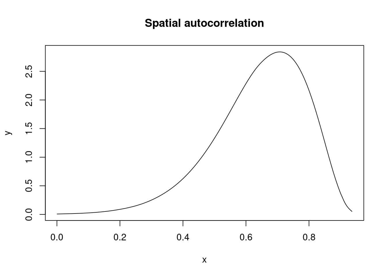
Summary of results
NY8$ICAR <- m.icar$summary.fitted.values[, "mean"]
NY8$BYM <- m.bym$summary.fitted.values[, "mean"]
NY8$LEROUX <- m.ler$summary.fitted.values[, "mean"]
NY8$SLM <- m.slm$summary.fitted.values[, "mean"]
spplot(NY8[syracuse, ],
c("FIXED.EFF", "IID.EFF", "ICAR", "BYM", "LEROUX", "SLM"),
col.regions = rev(magma(16))
)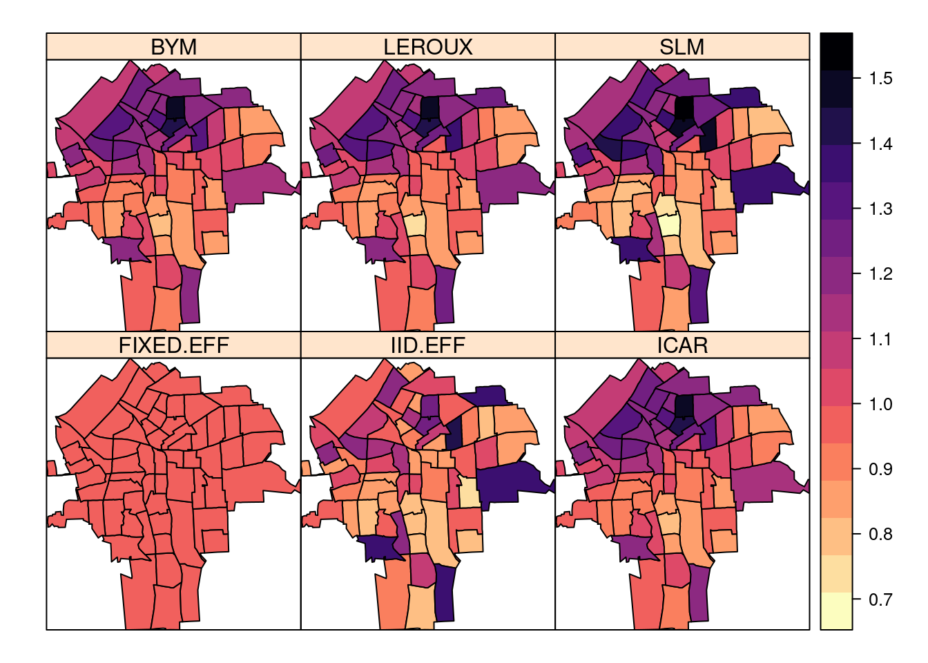
Note how spatial models produce smoother estimates of the relative risk.
In order to choose the best model, the model selection criteria computed above can be used:
| Marg. Lik. | DIC | WAIC | |
|---|---|---|---|
| FIXED | -480.2814 | 948.1198 | 949.0287 |
| IID | -478.6043 | 926.9295 | 932.6333 |
| ICAR | -685.6478 | 904.1253 | 906.7689 |
| BYM | -425.2479 | 903.4114 | 906.6138 |
| LEROUX | -474.4091 | 903.1453 | 906.1948 |
| SLM | -476.8145 | 902.3201 | 905.1892 |
References
Bivand, R., E. Pebesma and V. Gómez-Rubio (2013). Applied spatial data analysis with R. Springer-Verlag. New York.
Gómez-Rubio, V. (2020). Bayesian inference with INLA. CRC Press. Boca Raton, FL. https://becarioprecario.bitbucket.io/inla-gitbook
Rue, H., S. Martino and N. Chopin (2009). Approximate bayesian inference for latent Gaussian models by using integrated nested Laplace approximations. Journal of the royal statistical society: Series B (statistical methodology) 71(2): 319–392.
Waller, L. A. and C. A. Gotway (2004). Applied spatial statistics for public health data. John Wiley & Sons, Inc. Hoboken, New Jersey.