Stan is a probabilistic programming language for specifying statistical models. Stan provides full Bayesian inference for continuous-variable models through Markov Chain Monte Carlo methods such as the No-U-Turn sampler, an adaptive form of Hamiltonian Monte Carlo sampling. Penalized maximum likelihood estimates are calculated using optimization methods such as the limited memory Broyden-Fletcher-Goldfarb-Shanno algorithm. Stan can be called through R using the rstan package, and through Python using the pystan package. Both interfaces support sampling and optimization-based inference with diagnostics and posterior analysis. In this talk it is shown a brief glance about the main properties of Stan. It is also shown a couple of examples: the first one related with a simple Bernoulli model and the second one, about a Lotka-Volterra model based on ordinary differential equations.
What is Stan?
- Stan was created by Andrew Gelman and Bob Carpenter, with a development team consisting of 34 members.
- Stan is named in honor of Stanislaw Ulam (1909-1984), co-inventor of the Monte Carlo method.
- Stan is an imperative probabilistic programming language.
- A Stan program defines a probability model.
- It declares data and (constrained) parameter variables.
- It defines log posterior (or penalized likelihood).
- Stan inference: fits model to data and makes predictions.
- It can use Markov Chain Monte Carlo (MCMC) for full Bayesian inference.
- Or Variational Bayesian (VB) for approximate Bayesian inference.
- Or Maximum Likelihood Estimation (MLE) for penalized maximum likelihood estimation.
What does Stan compute?
- Draws from posterior distributions.
- MCMC sampling.
- Sequence of draws \(\theta_{(1)} ,\theta_{(2)}, \ldots, \theta_{(M)}\) where each draw \(\theta_{(i)}\) is marginally distributed according to the posterior \(p(\theta|y)\).
- Plot with histograms, kernel density estimates, etc.
You can see a quick look about rstan in its original wiki page.
Installing rstan
To run Stan in R, it is necessary to install rstan and a C++ compiler. On Windows, this means that Rtools is required, and you have to check whether the path (in Windows) is correctly fixed for all its binaries. If it is not the case, write in R:
install.packages(devtools)
library(devtools)
Sys.setenv(PATH = paste("C:\\Rtools\\bin", Sys.getenv("PATH"), sep=";"))
Sys.setenv(PATH = paste("C:\\Rtools\\mingw_64\\bin", Sys.getenv("PATH"), sep=";"))
Finally, install rstan:
install.packages(rstan)For more information about the frameworks which work with Stan (e.g.: Python) check this link.
Basic syntax in Stan
Defining the model
A Stan model is defined by six program blocks:
- Data (required).
- Transformed data.
- Parameters (required).
- Transformed parameters.
- Model (required).
- Generated quantities.
The data block reads external information.
data {
  int N;
  int x[N];
  int offset;
}
The transformed data block allows for preprocessing of the data.
transformed data {
  int y[N];
  for (n in 1:N)
    y[n] = x[n] - offset;
}
The parameters block defines the sampling space.
parameters {
  real<lower=0> lambda1;
  real<lower=0> lambda2;
}
The transformed parameters block allows for parameter processing before the posterior is computed.
transformed parameters {
  real<lower=0> lambda;
  lambda = lambda1 + lambda2;
}
In the model block we define our posterior distributions.
model {
  y ~ poisson(lambda);
  lambda1 ~ cauchy(0, 2.5);
  lambda2 ~ cauchy(0, 2.5);
}
Lastly, the generated quantities block allows for postprocessing.
generated quantities {
  int x_predict;
  x_predict = poisson_rng(lambda) + offset;
}
Types
Stan has two primitive types and both can be bounded.
- int is an integer type.
- real is a floating point precision type.
int<lower=1> N;

real<upper=5> alpha;
real<lower=-1,upper=1> beta;

real gamma;
real<upper=gamma> zeta;
Reals extend to linear algebra types.
vector[10] a;     // Column vector
matrix[10, 1] b;

row_vector[10] c; // Row vector
matrix[1, 10] d;
Arrays of integers, reals, vectors, and matrices are available.
real a[10];

vector[10] b;

matrix[10, 10] c;
Stan also implements a variety of constrained types.
simplex[5] theta;        // sum(theta) = 1

ordered[5] o;            // o[1] < ... < o[5]
positive_ordered[5] p;

corr_matrix[5] C;        // Symmetric and
cov_matrix[5] Sigma;     // positive-definite
More about Stan
All the typical control and loop statements are available, too.
if/then/else

for (i in 1:I)

while (i < I)
There are two ways to modify the posterior.
y ~ normal(0, 1);

target += normal_lpdf(y | 0, 1);

# Deprecated in new versions of Stan:
increment_log_posterior(log_normal(y, 0, 1))
And many sampling statements are vectorized.
parameters {
  real mu[N];
  real<lower=0> sigma[N];
}

model {
  // for (n in 1:N)
  // y[n] ~ normal(mu[n], sigma[n]);

  y ~ normal(mu, sigma);  // Vectorized version
}
The Bayesian approach
Probability is epistemic. For instance, John Stuart Mill (Logic 1882, Part III, Ch. 2) said:
[…] the probability of an event is not a quality of the event itself, but a mere name for the degree of ground which we, or someone else, have for expecting it. Every event is in itself certain, not probable; if we knew all, we should either know positively that it will happen, or positively that it will not.
[…] its probability to us means the degree of expectation of its occurrence, which we are warranted in entertaining by our present evidence.
Probabilities quantify uncertainty and we can consider that statistical reasoning is counterfactual.
Bayesian example with Stan: repeated binary trial model
As a first real approach to Stan and its syntax, we will start solving a small example in which the objective is, given a random sample drawn from a Bernoulli population, to estimate the posterior distribution of the missing parameter \(\theta \in \lbrack 0,1]\) (chance of success).
Step 1: Structure of the problem
In this example we will consider the following structure:
Data:
- \(N\in \{0,1,\ldots \}\), number of trials.
- \(y_{n}\in \{0,1\}\), result of trial n (known, modeled data).
Parameter:
\[\theta \in \lbrack 0,1]\]
- Prior distribution
\[p(\theta) = \mathrm{Uniform}(\theta|0,1) = 1\]
- Likelihood
\[p(y|\theta )=\prod_{n=1}^{N}\mathrm{Bernoulli}(y_{n}|\theta) = \prod_{n=1}^{N}\theta ^{y_{n}}(1-\theta )^{1-y_{n}}\]
- Posterior distribution
\[p(\theta |y)\propto p(\theta )p(y|\theta )\]
Step 2: Stan Program
We create the Stan program which we will call from R.
bern.stan =
"
data {
  int<lower=0> N;               // number of trials
  int<lower=0, upper=1> y[N];   // success on trial n
}

parameters {
  real<lower=0, upper=1> theta; // chance of success
}

model {
  theta ~ uniform(0, 1);        // prior
  y ~ bernoulli(theta);         // likelihood
}
"
Step 3: The data
In this case, instead of using a given data set, we will simulate a random sample to use in our example.
# Generate data
theta = 0.30
N = 20
y = rbinom(N, 1, 0.3)
y
## [1] 0 0 0 1 1 0 0 0 0 0 1 0 0 1 0 0 0 0 0 1Calculate MLE as the sample mean from data:
sum(y) / N## [1] 0.25Step 4: Bayesian Posterior using rstan
The final step is to obtain our estimation using Stan from R.
library(rstan)## Loading required package: ggplot2## Loading required package: StanHeaders## rstan (Version 2.18.2, GitRev: 2e1f913d3ca3)## For execution on a local, multicore CPU with excess RAM we recommend calling
## options(mc.cores = parallel::detectCores()).
## To avoid recompilation of unchanged Stan programs, we recommend calling
## rstan_options(auto_write = TRUE)fit = stan(model_code=bern.stan, data=list(y=y, N=N), iter=5000)##
## SAMPLING FOR MODEL '6dcfbccbf2f063595ccc9b93f383e221' NOW (CHAIN 1).
## Chain 1:
## Chain 1: Gradient evaluation took 7e-06 seconds
## Chain 1: 1000 transitions using 10 leapfrog steps per transition would take 0.07 seconds.
## Chain 1: Adjust your expectations accordingly!
## Chain 1:
## Chain 1:
## Chain 1: Iteration: 1 / 5000 [ 0%] (Warmup)
## Chain 1: Iteration: 500 / 5000 [ 10%] (Warmup)
## Chain 1: Iteration: 1000 / 5000 [ 20%] (Warmup)
## Chain 1: Iteration: 1500 / 5000 [ 30%] (Warmup)
## Chain 1: Iteration: 2000 / 5000 [ 40%] (Warmup)
## Chain 1: Iteration: 2500 / 5000 [ 50%] (Warmup)
## Chain 1: Iteration: 2501 / 5000 [ 50%] (Sampling)
## Chain 1: Iteration: 3000 / 5000 [ 60%] (Sampling)
## Chain 1: Iteration: 3500 / 5000 [ 70%] (Sampling)
## Chain 1: Iteration: 4000 / 5000 [ 80%] (Sampling)
## Chain 1: Iteration: 4500 / 5000 [ 90%] (Sampling)
## Chain 1: Iteration: 5000 / 5000 [100%] (Sampling)
## Chain 1:
## Chain 1: Elapsed Time: 0.012914 seconds (Warm-up)
## Chain 1: 0.013376 seconds (Sampling)
## Chain 1: 0.02629 seconds (Total)
## Chain 1:
##
## SAMPLING FOR MODEL '6dcfbccbf2f063595ccc9b93f383e221' NOW (CHAIN 2).
## Chain 2:
## Chain 2: Gradient evaluation took 2e-06 seconds
## Chain 2: 1000 transitions using 10 leapfrog steps per transition would take 0.02 seconds.
## Chain 2: Adjust your expectations accordingly!
## Chain 2:
## Chain 2:
## Chain 2: Iteration: 1 / 5000 [ 0%] (Warmup)
## Chain 2: Iteration: 500 / 5000 [ 10%] (Warmup)
## Chain 2: Iteration: 1000 / 5000 [ 20%] (Warmup)
## Chain 2: Iteration: 1500 / 5000 [ 30%] (Warmup)
## Chain 2: Iteration: 2000 / 5000 [ 40%] (Warmup)
## Chain 2: Iteration: 2500 / 5000 [ 50%] (Warmup)
## Chain 2: Iteration: 2501 / 5000 [ 50%] (Sampling)
## Chain 2: Iteration: 3000 / 5000 [ 60%] (Sampling)
## Chain 2: Iteration: 3500 / 5000 [ 70%] (Sampling)
## Chain 2: Iteration: 4000 / 5000 [ 80%] (Sampling)
## Chain 2: Iteration: 4500 / 5000 [ 90%] (Sampling)
## Chain 2: Iteration: 5000 / 5000 [100%] (Sampling)
## Chain 2:
## Chain 2: Elapsed Time: 0.01289 seconds (Warm-up)
## Chain 2: 0.012867 seconds (Sampling)
## Chain 2: 0.025757 seconds (Total)
## Chain 2:
##
## SAMPLING FOR MODEL '6dcfbccbf2f063595ccc9b93f383e221' NOW (CHAIN 3).
## Chain 3:
## Chain 3: Gradient evaluation took 3e-06 seconds
## Chain 3: 1000 transitions using 10 leapfrog steps per transition would take 0.03 seconds.
## Chain 3: Adjust your expectations accordingly!
## Chain 3:
## Chain 3:
## Chain 3: Iteration: 1 / 5000 [ 0%] (Warmup)
## Chain 3: Iteration: 500 / 5000 [ 10%] (Warmup)
## Chain 3: Iteration: 1000 / 5000 [ 20%] (Warmup)
## Chain 3: Iteration: 1500 / 5000 [ 30%] (Warmup)
## Chain 3: Iteration: 2000 / 5000 [ 40%] (Warmup)
## Chain 3: Iteration: 2500 / 5000 [ 50%] (Warmup)
## Chain 3: Iteration: 2501 / 5000 [ 50%] (Sampling)
## Chain 3: Iteration: 3000 / 5000 [ 60%] (Sampling)
## Chain 3: Iteration: 3500 / 5000 [ 70%] (Sampling)
## Chain 3: Iteration: 4000 / 5000 [ 80%] (Sampling)
## Chain 3: Iteration: 4500 / 5000 [ 90%] (Sampling)
## Chain 3: Iteration: 5000 / 5000 [100%] (Sampling)
## Chain 3:
## Chain 3: Elapsed Time: 0.012875 seconds (Warm-up)
## Chain 3: 0.01241 seconds (Sampling)
## Chain 3: 0.025285 seconds (Total)
## Chain 3:
##
## SAMPLING FOR MODEL '6dcfbccbf2f063595ccc9b93f383e221' NOW (CHAIN 4).
## Chain 4:
## Chain 4: Gradient evaluation took 3e-06 seconds
## Chain 4: 1000 transitions using 10 leapfrog steps per transition would take 0.03 seconds.
## Chain 4: Adjust your expectations accordingly!
## Chain 4:
## Chain 4:
## Chain 4: Iteration: 1 / 5000 [ 0%] (Warmup)
## Chain 4: Iteration: 500 / 5000 [ 10%] (Warmup)
## Chain 4: Iteration: 1000 / 5000 [ 20%] (Warmup)
## Chain 4: Iteration: 1500 / 5000 [ 30%] (Warmup)
## Chain 4: Iteration: 2000 / 5000 [ 40%] (Warmup)
## Chain 4: Iteration: 2500 / 5000 [ 50%] (Warmup)
## Chain 4: Iteration: 2501 / 5000 [ 50%] (Sampling)
## Chain 4: Iteration: 3000 / 5000 [ 60%] (Sampling)
## Chain 4: Iteration: 3500 / 5000 [ 70%] (Sampling)
## Chain 4: Iteration: 4000 / 5000 [ 80%] (Sampling)
## Chain 4: Iteration: 4500 / 5000 [ 90%] (Sampling)
## Chain 4: Iteration: 5000 / 5000 [100%] (Sampling)
## Chain 4:
## Chain 4: Elapsed Time: 0.012823 seconds (Warm-up)
## Chain 4: 0.014169 seconds (Sampling)
## Chain 4: 0.026992 seconds (Total)
## Chain 4:print(fit, probs=c(0.1, 0.9))## Inference for Stan model: 6dcfbccbf2f063595ccc9b93f383e221.
## 4 chains, each with iter=5000; warmup=2500; thin=1;
## post-warmup draws per chain=2500, total post-warmup draws=10000.
##
## mean se_mean sd 10% 90% n_eff Rhat
## theta 0.27 0.00 0.09 0.16 0.39 3821 1
## lp__ -13.40 0.01 0.73 -14.25 -12.90 3998 1
##
## Samples were drawn using NUTS(diag_e) at Tue Jan 22 11:25:43 2019.
## For each parameter, n_eff is a crude measure of effective sample size,
## and Rhat is the potential scale reduction factor on split chains (at
## convergence, Rhat=1).# Extracting the posterior draws
theta_draws = extract(fit)$theta
# Calculating posterior mean (estimator)
mean(theta_draws)## [1] 0.2715866# Calculating posterior intervals
quantile(theta_draws, probs=c(0.10, 0.90))## 10% 90%
## 0.1569165 0.3934832theta_draws_df = data.frame(list(theta=theta_draws))
plotpostre = ggplot(theta_draws_df, aes(x=theta)) +
geom_histogram(bins=20, color="gray")
plotpostre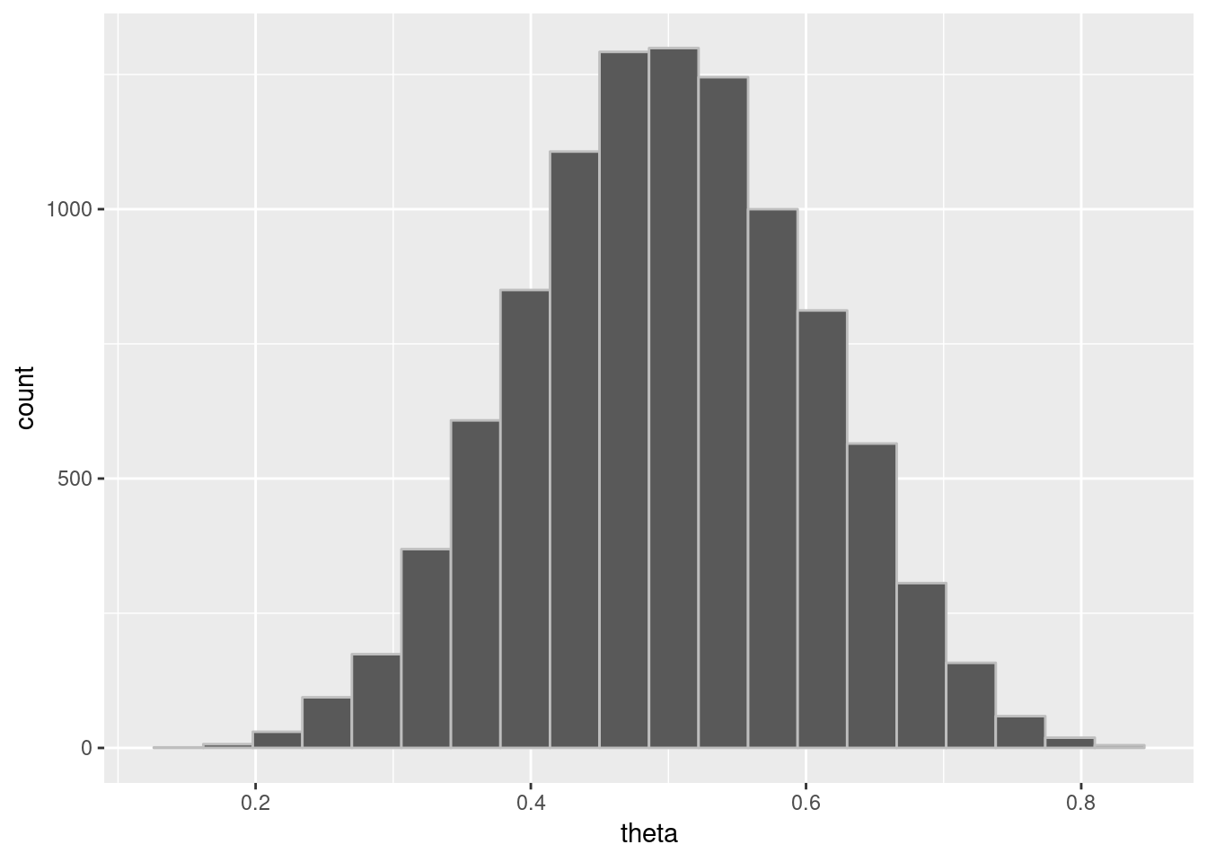
RStan: MAP, penalized MLE
Stan’s optimization for estimation; two views:
- max posterior mode, also known as max a posteriori (MAP).
- max penalized likelihood (MLE).
library(rstan)
N = 5
y = c(0, 1, 1, 0, 0)

model = stan_model(model_code=bern.stan)
mle = optimizing(model, data=c("N", "y"))

print(mle, digits=2)
## $par
## theta
## 0.4
##
## $value
## [1] -3.4
##
## $return_code
## [1] 0Lotka-Volterra’s Model
- Lotka (1925) and Volterra (1926) formulated parametric differential equations that characterize the oscillating populations of predators and preys.
- A statistical model to account for measurement error and unexplained variation uses the deterministic solutions to the Lotka-Volterra equations as expected population sizes.
- Full Bayesian inference may be used to estimate future (or past) populations.
- Stan is used to encode the statistical model and perform full Bayesian inference to solve the inverse problem of inferring parameters from noisy data.
See full reference: Stan and Lotka-Volterra models.
In this example, we want to fit the model to Canadian lynx predator and snowshoe hare prey with respective populations between 1900 and 1920, based on the number of pelts collected annually by the Hudson’s Bay Company.
Notation and mathematical model
We denote \(u(t)\) and \(v(t)\) as the prey and predator population respectively. The differential equations that relate them are:
\[\frac{d}{dt}u = (\alpha -\beta v)u\]
\[\frac{d}{dt}v=(-\gamma +\delta u)v\]
Here:
- \(\alpha\): prey growth, intrinsic.
- \(\beta\): prey shrinkage due to predation.
- \(\gamma\): predator shrinkage, intrinsic.
- \(\delta\): predator growth from predation.
Lotka-Volterra in Stan
real[] dz_dt(data real t,       // time
  real[] z,                     // system state
  real[] theta,                 // parameters
  data real[] x_r,              // real data
  data int[] x_i)               // integer data
{
  real u = z[1];                // extract state
  real v = z[2];
  real alpha = theta[1];
  real beta = theta[2];
  real gamma = theta[3];
  real delta = theta[4];

  real du_dt = (alpha - beta * v) * u;
  real dv_dt = (-gamma + delta * u) * v;
  return { du_dt, dv_dt };
}
Known variables are observed:
- \(y_{n,k}\): denotes species \(k\) at times \(t_{n}\) for \(n \in 0:N\)
Unknown variables must be inferred (inverse problem):
- Initial state: \(z_{k}^{init}\): initial population for \(k\).
- Subsequent states \(z_{n,k}\): population \(k\) at time \(t_{n}\).
- Parameters \(\alpha\), \(\beta\), \(\gamma\), \(\delta > 0\).
Likelihood assumes errors are proportional (not additive):
\[y_{n,k}\sim \mathrm{LogNormal}(\hat{z}_{n,k}, \sigma_{k})\]
Equivalently:
\[\log y_{n,k} = \log \widehat{z}_{n,k} + \epsilon_{n,k}\]
with
\[\epsilon_{n,k} \sim \mathrm{Normal}(0, \sigma_{k})\]
Creating the model
Variables for known constants and observed data.
data {
  int<lower = 0> N;       // num measurements
  real ts[N];             // measurement times > 0
  real y0[2];             // initial pelts
  real<lower=0> y[N,2];   // subsequent pelts
}
Variables for unknown parameters.
parameters {
  real<lower=0> theta[4];    // alpha, beta, gamma, delta
  real<lower=0> z0[2];       // initial population
  real<lower=0> sigma[2];    // scale of prediction error
}
Prior distribution and likelihood.
model {
  // priors
  sigma ~ lognormal(0, 0.5);
  theta[{1, 3}] ~ normal(1, 0.5);
  theta[{2, 4}] ~ normal(0.05, 0.05);
  z0[1] ~ lognormal(log(30), 5);
  z0[2] ~ lognormal(log(5), 5);

  // likelihood (lognormal)
  for (k in 1:2) {
    y0[k] ~ lognormal(log(z0[k]), sigma[k]);
    y[ , k] ~ lognormal(log(z[, k]), sigma[k]);
  }
}
Solution to the differential equations. We have to define variables for populations predicted by ode, given:
- System function (
dz_dt), initial populations (z0). - Initial time (
0.0), solution times (ts). - Parameters (
theta), data arrays. - Tolerances (
1e-6, 1-e4), max iterations (1e3).
transformed parameters {
  real z[N, 2] = integrate_ode_rk45(
    dz_dt, z0, 0.0, ts, theta, rep_array(0.0, 0),
    rep_array(0, 0), 1e-6, 1e-4, 1e3);
}
Lotka-Volterra Parameter estimation
fit = stan(lotka-volterra.stan, data=lynx_hare_data)

print(fit, c("theta", "sigma"), probs=c(0.1, 0.5, 0.9))
It is obtained, for example:
               mean  se_mean   sd  10%  50%  90%  n_eff  Rhat
## theta[1]    0.55    0     0.07 0.46 0.54 0.64   1168     1
## theta[2]    0.03    0     0.00 0.02 0.03 0.03   1305     1
## theta[3]    0.80    0     0.10 0.68 0.80 0.94   1117     1
## theta[4]    0.02    0     0.00 0.02 0.02 0.03   1230     1
## sigma[1]    0.29    0     0.05 0.23 0.28 0.36   2673     1
## sigma[2]    0.29    0     0.06 0.23 0.29 0.37   2821     1
Analysis of the obtained results:
- Rhat near 1 signals convergence; n_eff is effective sample size.
- 10%, … posterior quantiles; e.g. \(P[\alpha \in (0.46,0.64)|y]=0.8\).
- Posterior mean is a Bayesian point estimate: \(\alpha = 0.55\).
- Standard error in posterior mean estimate is 0 (with rounding).
- Posterior standard deviation of \(\alpha\) is 0.07.
Full program to run
file = "https://raw.githubusercontent.com/stan-dev/example-models/master/knitr/lotka-volterra/hudson-bay-lynx-hare.csv"
# https://github.com/bblais/Systems-Modeling-Spring-2015-Notebooks/blob/master/data/Lynx%20and%20Hare%20Data/lynxhare.csv

lynx_hare_df = read.csv(file, header=TRUE, comment.char="#")
# lynx_hare_df

N = length(lynx_hare_df$Year) - 1
ts = 1:N
y_init = c(lynx_hare_df$Hare[1], lynx_hare_df$Lynx[1])
y = as.matrix(lynx_hare_df[2:(N + 1), 2:3])
y = cbind(y[ , 2], y[ , 1]); # hare, lynx order
lynx_hare_data = list(N, ts, y_init, y)

library(rstan)

thething = "
functions {
  real[] dz_dt(real t, real[] z, real[] theta,
             real[] x_r, int[] x_i) {
      real u = z[1];
      real v = z[2];

      real alpha = theta[1];
      real beta = theta[2];
      real gamma = theta[3];
      real delta = theta[4];

      real du_dt = (alpha - beta * v) * u;
      real dv_dt = (-gamma + delta * u) * v;
      return { du_dt, dv_dt };
    }
}

data {
  int<lower = 0> N;           // num measurements
  real ts[N];                 // measurement times > 0
  real y_init[2];             // initial measured population
  real<lower = 0> y[N, 2];    // measured population at measurement times
}

parameters {
  real<lower = 0> theta[4];   // theta = {alpha, beta, gamma, delta}
  real<lower = 0> z_init[2];  // initial population
  real<lower = 0> sigma[2];   // error scale
}

transformed parameters {
  real z[N, 2]
    = integrate_ode_rk45(dz_dt, z_init, 0, ts, theta,
                         rep_array(0.0, 0), rep_array(0, 0),
                         1e-6, 1e-5, 1e3);
}

model {
  theta[{1, 3}] ~ normal(1, 0.5);
  theta[{2, 4}] ~ normal(0.05, 0.05);
  sigma ~ lognormal(-1, 1);
  z_init ~ lognormal(log(10), 1);
  for (k in 1:2) {
    y_init[k] ~ lognormal(log(z_init[k]), sigma[k]);
    y[ , k] ~ lognormal(log(z[, k]), sigma[k]);
  }
}
"

fit = stan(model_code=thething, data=lynx_hare_data, iter=5000, chains=3, cores=3)

print(fit, pars=c("theta", "sigma", "z_init"),
      probs=c(0.1, 0.5, 0.9), digits = 3)
Other references and examples of Stan
- Andrew Gelman has a blog about
rstanthat shows examples to run in RStudio Cloud. But I had problems to run these codes in the Cloud… :-( - Example Session in RStudio Cloud.
- All examples of his blog can be downloaded from GitHub.