Network analysis offers a perspective of the data that broadens and enriches any investigation. Many times we deal with data in which the elements are related, but we have them in a tabulated format that is difficult to import into network analysis tools.
Relationship data require a definition of nodes and connections. Both parts have different structures and it is not possible to structure them in a single table, at least two would be needed. Data analysis tools define different input formats, one of them is GDF, which is characterized by its simplicity and versatility.
In this session, we will see how we can extract the relationships between elements of a file in CSV format to generate a file in GDF format to work with Gephi.
Introduction
One of the most used network analysis tools is Gephi. It is a desktop application that allows us to analyse a network in depth and visualize it. It provides a set of functions to filter nodes and edges or calculate network parameters or apply different layouts or give size and colour to nodes depending on different attributes.
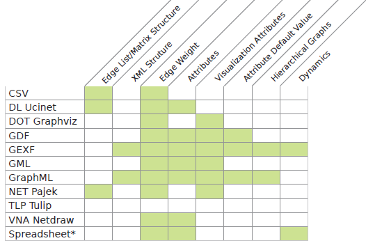
Gephi supports a set of formats with which it is possible to perform more or less functions. The format with more features is GEXF but it has an XML structure that generates large files. When we work with very large graphs, size matters. The GDF Format is simple, compact and versatile. It allows us to work with attributes that are a complement that can be combined with the analysis of the topology of the network.

As Gephi said:
GDF is built like a database table or a coma separated file (CSV). It supports attributes to both nodes and edges. A standard file is divided in two sections, one for nodes and one for edges. Each section has a header line, which basically is the column title. Each element (i.e. node or edge) is on a line and values are separated by coma. The GDF format is therefore very easy to read and can be easily converted from CSV.
This is a basic example of a GDF file, in a first part it defines the nodes and in a second the connections:
nodedef>name VARCHAR,label VARCHAR
s1,Site number 1
s2,Site number 2
s3,Site number 3
edgedef>node1 VARCHAR,node2 VARCHAR
s1,s2
s2,s3
s3,s2
s3,s1
The steps to extract relationships from a CSV file and generate a file in GDF format are:
- Define the parameters for the extraction of related data.
- Define the data structures for the transformation.
- Import the data from a file in CSV format and store the data in the structures.
- Sort data according to connections.
- Prepare the data for the GDF format.
- Generate the file in GDF format.
Define the parameters for the extraction of related data
A set of parameters are defined so this converter can be adapted to different cases. We must specify what information will be taken from the file in CSV format, where we will leave the result and the graph type.
library("readr")
library("hash")
library("stringr")

source <- 3                            # Column number of source entity
target <- 9                            # Column number of target entity
source_attribs <- c(5, 6, 11, 12, 13)  # Column numbers of attribs
null_attrib <- rep(NA, 5)              # Default value for entities without attributes
name_attribs <- c("app", "location", "hastag", "lang", "create at") # Attrib names
name_file_csv <- "rstudio_RTs.csv"     # Name of the input file in CSV format
name_file_gdf <- "rstudio_RTs.gdf"     # Name of the output file in GDF format
directed <- TRUE                       # Indicates whether the graph is directed or not
The sample CSV file can be found here.
Define the data structures for the transformation
In order to store the data, dynamic structures are needed to allow data to be added as they appear. The hash tables were chosen because they are the most appropriate for this case. Hash tables will be used to store nodes and connections.
hash_nodes <- hash()
hash_links <- hash()
hash_links_in <- hash()
hash_links_out <- hash()
hash_connections <- hash()
hash_connections_attrib <- hash()
num_attribs <- length(source_attribs)
Import the data from a file in CSV format and store the data in the structures
Import data reading the CSV file and run it row by row to store the nodes and connections in the hash tables.
Related entities can appear multiple times, as a source or as a target. When an entity appears for the first time, it is stored in the hash_nodes table. Attributes are associated to source entities and null attributes to target entities. It is a criterion that assumes this algorithm, but there could be others. If an entity appears the first time as a target, it will be assigned the null attributes, but if it appears later as a source, the null attributes will be replaced by theirs.
For each entity, the number of total links (hash_links), the number of inbound links (hash_links_in) and the number of outbound links (hash_links) are counted. This is done to allow ordering the nodes from greater to lesser degree when generating the file in GDF format.
For each origin-target entity pair, the number of times that the relation appears (hash_connections) and the attributes (hash_connections_attrib) are stored. In the first case, we get the weight of the relationship and, in the second, we get the associated attributes.
table_csv <- read_csv2(name_file_csv)
num_rows <- nrow(table_csv)
num_cols <- ncol(table_csv)
for (i in 1:num_rows)
{
  node_source <- table_csv[[i, source]]
  node_target <- table_csv[[i, target]]
  print(i)
  node_source_attribs <- null_attrib
  # The attributes are stored and the ',' character is changed by '-'. to avoid confict in the GDF format
  for (j in 1:num_attribs)
  {
    k <- source_attribs[[j]]
    raw_attrib <- table_csv[[i, k]]
    cooked_attrib <- str_replace_all(raw_attrib, ",", "-")
    node_source_attribs[[j]] <- cooked_attrib
  }
  # If a source node appears for the first time, store with attributes
  if (!(has.key(node_source, hash_nodes)))
  {
    hash_nodes[[node_source]] <- node_source_attribs
    hash_links[[node_source]] <- 0
    hash_links_in[[node_source]] <- 0
    hash_links_out[[node_source]] <- 0
  }
  # If the source node exists and has null attributes, store its own
  else
  {
    node_source_attribs_old <- hash_nodes[[node_source]]
    if (identical(node_source_attribs_old, null_attrib))
      hash_nodes[[node_source]] <- node_source_attribs
  }
  # Check that target node exists
  if (!(is.na(node_target)))
  {
    # If a target node appears for the first time, store with null attributes
    if (!(has.key(node_target, hash_nodes)))
    {
      hash_nodes[[node_target]] <- null_attrib
      hash_links[[node_target]] <- 0
      hash_links_in[[node_target]] <- 0
      hash_links_out[[node_target]] <- 0
    }
    par_nodes <- paste(node_source, node_target)
    # If a pair of nodes appears for the first time related, store relation
    if (!(has.key(par_nodes, hash_connections)))
    {
      hash_connections[[par_nodes]] <- 0
      hash_connections_attrib[[par_nodes]] <- node_source_attribs
    }
    # In all cases, increase the number of connections
    hash_connections[[par_nodes]] <- hash_connections[[par_nodes]] + 1
    hash_links[[node_source]] <- hash_links[[node_source]] + 1
    hash_links_out[[node_source]] <- hash_links_out[[node_source]] + 1
    hash_links[[node_target]] <- hash_links[[node_target]] + 1
    hash_links_in[[node_target]] <- hash_links_in[[node_target]] + 1
  }
}
Sort data according to connections
The hash table object does not have the sort method, but has one to convert it into a list. Once we have converted the hash_links and hash_connections into a list, we sort them down by number of connections.
list_links <- as.list.hash(hash_links)
list_link_order <- list_links[order(unlist(list_links), decreasing=TRUE)]
list_connections <- as.list.hash(hash_connections)
list_connections_order <- list_connections[order(unlist(list_connections), decreasing=TRUE)]
Prepare the data for the GDF format
In this step we place in GDF format nodes and links in descending order by number of connections.
In the GDF format, the only data required for the definition of nodes is the name of the node, but attributes can be added. In this case, three fixed attributes are included, which are the total number of links, the number of inbound links and the number of outbound links. Since the GDF format is readable, these attributes allow getting an idea of the most relevant nodes even before importing them into Gephi. The attributes configured in the parameters are also added.
The information of the nodes is stored in a matrix sized in rows by the number of nodes and in columns by the number of attributes configured plus four.
For the definition of links only the source and target nodes are required, but we can also expand them with attributes. In this case we add the weight of the relation, a boolean variable to indicate if the graph is directed or not (by default it is not directed) and the attributes configured in the parameters.
The information of the links is stored in a matrix dimensioned in rows by the number of pairs of connections and in columns by the number of attributes configured plus four.
# Definition of nodes
num_nodes <- length(list_links)
table_nodes <- matrix(nrow=num_nodes, ncol=num_attribs+4)
num_nodes_connected <- 0
for(i in 1:num_nodes)
{
  name_node <- names(list_link_order)[i]
  if (hash_links[[name_node]] > 0)
  {
    num_nodes_connected <- num_nodes_connected + 1
    table_nodes[i, 1] <- name_node
    table_nodes[i, 2] <- hash_links[[name_node]]
    table_nodes[i, 3] <- hash_links_in[[name_node]]
    table_nodes[i, 4] <- hash_links_out[[name_node]]
    node_attrib <- hash_nodes[[name_node]]
    for (j in 1:num_attribs)
      table_nodes[i, 4+j] <- node_attrib[[j]]
  }
}
# Only connected nodes are considered
k <- num_attribs + 4
table_nodes <- table_nodes[1:num_nodes_connected, 1:k]

# Definition of links
num_connections <- length(list_connections)
table_connections <- matrix(nrow=num_connections, ncol=num_attribs+4)
for(i in 1:num_connections)
{
  name_conexion <- names(list_connections_order)[i]
  source_target <- strsplit(name_conexion, " ")
  table_connections[i, 1] <- source_target[[1]][1]
  table_connections[i, 2] <- source_target[[1]][2]
  table_connections[i, 3] <- list_connections_order[[i]]
  table_connections[i, 4] <- directed
  connection_attrib <- hash_connections_attrib[[name_conexion]]
  for (j in 1:num_attribs)
    table_connections[i, 4+j] <- connection_attrib[[j]]
}
Generate the file in GDF format
The last step is to write the file in GDF format. We will only have to add the headers before writing the information of the nodes and links.
# Definition of nodes
head_nodes <- "nodedef>name VARCHAR,links INT,Links_in INT,links_out INT"
for (j in 1:num_attribs)
{
  attrib_type <- paste(name_attribs[[j]], "VARCHAR", sep = " ")
  head_nodes <- paste(head_nodes, attrib_type, sep = ",")
}
write.table(head_nodes, file = name_file_gdf, append = FALSE, quote = FALSE, sep = ",",
            eol = "\n", na = "NA", dec = ".", row.names = FALSE,
            col.names = FALSE, qmethod = c("escape", "double"),
            fileEncoding = "UTF-8")
write.table(table_nodes, file = name_file_gdf, append = TRUE, quote = FALSE, sep = ",",
            eol = "\n", na = "NA", dec = ".", row.names = FALSE,
            col.names = FALSE, qmethod = c("escape", "double"),
            fileEncoding = "UTF-8")

# Definition of links
head_arcs <- "edgedef>node1 VARCHAR,node2 VARCHAR, weight INT, directed BOOLEAN"
for (j in 1:num_attribs)
{
  attrib_type <- paste(name_attribs[[j]], "VARCHAR", sep = " ")
  head_arcs <- paste(head_arcs, attrib_type, sep = ",")
}
write.table(head_arcs, file = name_file_gdf, append = TRUE, quote = FALSE, sep = ",",
            eol = "\n", na = "NA", dec = ".", row.names = FALSE,
            col.names = FALSE, qmethod = c("escape", "double"),
            fileEncoding = "UTF-8")
write.table(table_connections, file = name_file_gdf, append = TRUE, quote = FALSE, sep = ",",
            eol = "\n", na = "NA", dec = ".", row.names = FALSE,
            col.names = FALSE, qmethod = c("escape", "double"),
            fileEncoding = "UTF-8")
The resulting GDF file can be found here, and also the complete R code is available in a standalone script.
Example
The data has been obtained with the tool t-hoarder_kit, which allows downloading data through the Twitter API. With it, a query of the tweets that mentioned the @rstudio profile has been made. From the data downloaded in CSV format, the most relevant columns have been selected to facilitate the visibility of the tables.
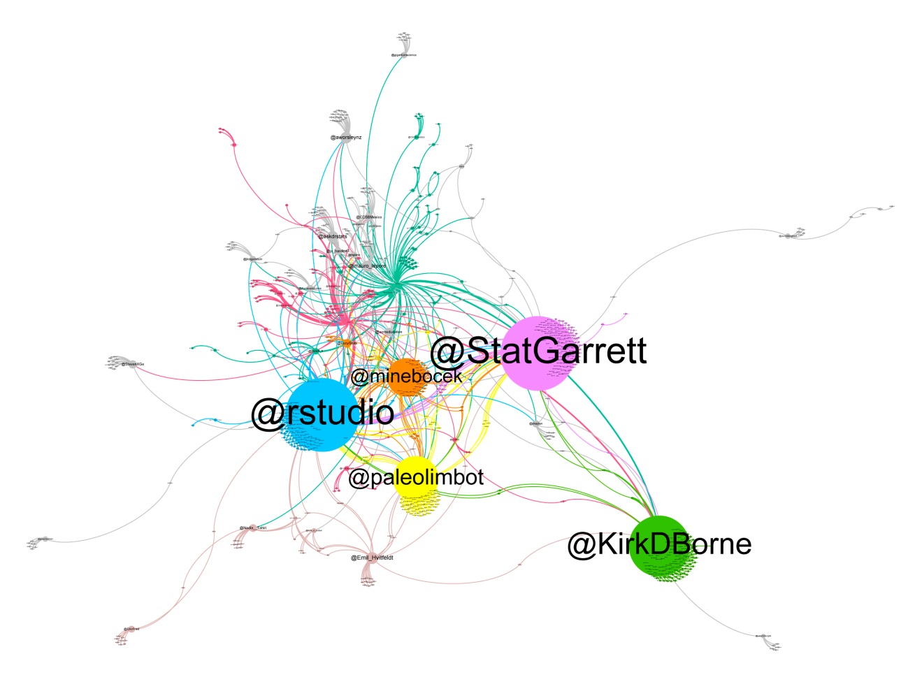
Once the file in CSV format has been converted to a file in GDF format with the RT relation, this is the visualization of the graph with Gephi. (tweets from 2019-05-27 to 2019-06-06)
