Do you want to know how to make elegant and simple reproducible presentations? In this talk, we are going to explain how to do presentations in different output formats using one of the easiest and most exhaustive statistical software, R. Now, it is possible create Beamer, PowerPoint, or HTML presentations, including R code, \(\LaTeX\) equations, graphics, or interactive content.
After the tutorial, you will be able to create R presentations on your own with R Markdown in RStudio. But don’t worry if you don’t know a lot of R Markdown, because it’s really simple to use it with RStudio and you will discover the keys to master the language.
We have several options to create amazing technical presentations in pdf format with tools like PowerPoint or \(\LaTeX\). But the truth is that when we want to generate a full and complete document with graphs, code, and text, then we invest more time in the appearance than in the content itself, or learning how to add content easily. So here I want to show you a good alternative using R. The best feature R has is the flexibility and simplicity of the code to reproduce amazing presentations with little work. To achieve it, R uses Markdown. But, what is exactly Markdown?
What is Markdown?
Markdown is a simple language to write web-based content easy both for writing and reading. The key is that it can be converted to many output formats with a simplified syntax.
Basics of Markdown
Here you have a summary guide of the main style syntax.
Headers
# H1
## H2
### H3
#### H4
##### H5
###### H6

Alternatively, for H1 and H2, an underline-ish style:

Alt-H1
======

Alt-H2
------
Emphasis
*italics* or _italics_.

**bold** or __bold__.

~~Strikethrough~~
Lists
1. First ordered list item
2. Another item

* Unordered list can use asterisks
- Or minuses
+ Or pluses
Links
[I'm an inline-style link](https://www.google.com)Images
Inline-style:
Code and syntax highlighting
Inline `code` has `back-ticks around` it.```python
s = "Python syntax highlighting"
print s
```Blockquotes
> Blockquotes are very handy in emails to emulate reply text.TeX Formula
$-b \pm \sqrt{b^2 - 4ac} \over 2a$Besides these basics, you can to add tables, rulers, links to videos, HTML code, etc. To know more visit the creator’s web site: https://daringfireball.net/projects/markdown/ or this cheatsheet https://github.com/adam-p/markdown-here/wiki/Markdown-Cheatsheet.
R has a specific file format for this type of documents .Rmd. R Markdown has an online book really useful and detailed here https://bookdown.org/yihui/rmarkdown/. This tool let you build different type of documents like the next ones:
- Documents: HTML, \(\LaTeX\)/PDF, Microsoft Word, Tufte-style handouts
- Interactive documents: HTML Widgets, Shiny
- Dashboards: Gauges, values boxes, HTML Widgets, Shiny, Storyboard
- Books: HTML, PDF, EPUB
- Web sites
- JSS templates, R Journal, Skeleton, CV
- Package Vignettes
- Presentations: Beamer, Slidy, ioslides, reveal.js, xaringan
In the next link, you will find some examples of each one https://rmarkdown.rstudio.com/gallery.HTML. And in this cheatsheet, a good summary of R Markdown is presented https://rmarkdown.rstudio.com/lesson-15.HTML.
How to start
The first step is to get R and RStudio, and install the package rmarkdown with the code
install.packages("rmarkdown")In the last versions you can directly create presentations going to File -> New File -> R Presentation. Then, a .RPres document is going to be created. This is the simplest, really simplest, way to start but my advice is to go quickly to the next step if you want more flexibility in the slides and final appearance.
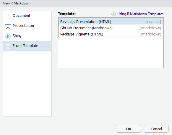
So going to File -> New File -> R Markdown and selecting the option Presentation, you are going to have different options to create your slides. Selecting any of them, a file like this is automatically generated:
Depending on the final style of the output there are different output options. In the next points, we are going to explain in detail the main features of all them.
- ioslides: the option
output: ioslides_presentation - slidy: the option
output: slidy_presentation - beamer: the option
output: beamer_presentation
The R Markdown file
Header
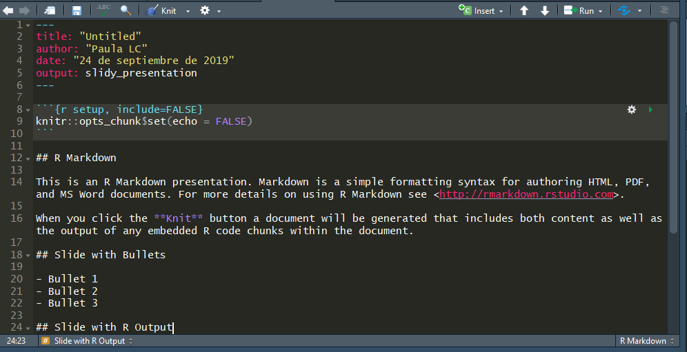
The header is the R Markdown document part where you can set the title, the author, the date, and the output as the image shows:
---
title: "Mastering R presentations"
author: "Paula LC"
date: "2019-09-24"
output: ioslides_document
---
But at the same time, other options can be determined as follows:
---
title: "Mastering R presentations"
author: "Paula LC"
date: "2019-09-24"
output:
  ioslides_presentation:
    incremental: false
    self-included: true
---
Content
Once the header is completed, you can add any kind of content that you can practically imagine: R code, equations, charts, images, videos etc. In the next points we are going to see how to add each type of content.
R Chunks
In addition to plain text, headers and other Markdown elements, you have the option of inserting R code which will be executed every time you run the file. These parts of the document are called R chunks. To insert an R Chunk you can use RStudio toolbar Insert button or the keyboard shortcut Ctrl + Alt + I on Windows and Cmd + Option + I on macOS.
There are a lot of options referring to how to include tables, text output, figures, etc. For example, to add the option to show in the output the R code before the results you have to add between the brackets {r } the option echo as follows {r echo=TRUE}. By default, the code is not shown.
More options:
- cache: cache results for future knits (default = FALSE)
- cache.path: directory to save cached results in (default = “cache/”)
- child: file(s) to knit and then include (default = NULL)
- collapse: collapse all output into single block (default = FALSE)
- comment: prefix for each line of results (default = ‘##’)
- dependson: chunk dependencies for caching (default = NULL)
- echo: Display code in output document (default = TRUE)
- engine: code language used in chunk (default = ‘R’)
- error: Display error messages in doc (TRUE) or stop render when errors occur (FALSE) (default = FALSE)
- eval: Run code in chunk (default = TRUE)
- message: display code messages in document (default = TRUE)
- results=asis: passthrough results
- results=hide: do not display results
- results=hold: put all results below all code
- tidy: tidy code for display (default = FALSE)
- warning: display code warnings in document (default = TRUE)
- fig.align: ‘lef’, ‘right’, or ‘center’ (default = ‘default’)
- fig.cap: figure caption as character string (default = NULL)
- fig.height, fig.width: Dimensions of plots in inches
- highlight: highlight source code (default = TRUE)
- include: Include chunk in doc after running (default = TRUE)
In the next link you can find more details about R chunks: https://bookdown.org/yihui/rmarkdown/r-code.HTML
Equations
There is the chance to add equations to your presentations with MathJax scripts. These are included in HTML documents for rendering \(\LaTeX\) and MathML equations. To control how MathJax is included you have the next options:
defaultto use an HTTPS URL from a CDN host (currently provided by RStudio)local: to use a local version of MathJax (which is copied into the output directory). Note that when using “local” you also need to set the self_contained option to false.- URL indicating the location to load MathJax
nullto exclude MathJax entirely.
For example, to use a local copy of MathJax:
---
title: "Example"
output:
  ioslides_document:
    mathjax: local
    self_contained: false
---
To use a self-hosted copy of MathJax:
---
title: "Example"
output:
  ioslides_document:
    mathjax: "http://example.com/MathJax.js"
---
Tables
You have four options to add tables. First one, directly from R Markdown
Colons can be used to align columns.

| Tables        | Are           | Cool  |
| ------------- |:-------------:| -----:|
| col 3 is      | right-aligned | $1600 |
| col 2 is      | centered      |   $12 |
| zebra stripes | are neat      |    $1 |
or the next ones, from R code with the libraries knitr, xtable, or stargazer.
data <- faithful[1:4, ]
knitr::kable(data, caption = 'Table with kable')

data <- faithful[1:4, ]
print(xtable::xtable(data, caption = 'Table with xtable'), type = 'HTML',
      HTML.table.attributes = 'border=0')

data <- faithful[1:4, ]
stargazer::stargazer(data, type = 'HTML', title = 'Table with stargazer')
Interactive graphs
In R there are a lot of packages to create interactive graphs. Highcharter is one of them, as well as the well-known HTMLwidgets. Here we have an example of a highcharter graph.
library(highcharter)
highchart() %>%
  hc_title(text = "Scatter chart with size and color") %>%
  hc_add_series(mtcars, "point", hcaes(wt, mpg, size=drat, color=hp)) %>%
  widgetframe::frameWidget()
Presentation formats
We just explored the different contents and parts of our R Markdown document. Let’s see what type of output format we can obtain.
Ioslides
Ioslides is a nice R presentation format characterized by the simplicity of the result. There are some features specific from ioslides, such as the display mode
f: enable fullscreen modew: toggle widescreen modeo: enable overview modeh: enable code highlight modep: show presenter notes
or the incremental bullets:
---
output:
  ioslides_presentation:
    incremental: true
---
Moreover, you can change the presentation size, the text size, or even the transition speed in the header of the document. Specifically, for the transition speed you can set the number of seconds for each slide or use the standard options: default, slower, faster.
---
output:
  ioslides_presentation:
    widescreen: true
    smaller: true
    transition: slower
---
For another hand, there is a quick way to add a background image without editing the CSS file,
## {data-background="my_background.png"}But if you want to add specific style changes to your presentation, I recommend you to edit the CSS file and add it to the header of the RMarkdown document:
---
output:
  ioslides_presentation:
    css: styles.css
---
One of the disadvantages of ioslides is that customization is limited compared with other output formats. At the end of this tutorial we explain how to modify by your own a CSS file.
Slidy
Slidy has more flexibility than ioslides as to appearance and style. Now we are going to see some of the main special features that slidy has.
There is the chance to change the display mode with the next shortcuts;
c: Show table of contentsc: Toggles the display of the footera: Toggles display of current vs all slides (useful for printing handouts)s: Make fonts smallerb: Make fonts larger
And we can adjust the font directly in the header of the document without editing the CSS file:
---
output:
  slidy_presentation:
    font_adjustment: -1
---
You will find other interesting features of slidy such as the countdown timer in the footer or the customized footer text that can be easily added with the options duration and footer.
Slidy themes
In slidy, there are different Boostrap themes to use drawn from the Bootswatch theme library. The themes are default, cerulean, journal, flatly, darkly, readable, spacelab, united, cosmo, lumen, paper, sandstone, simplex, and yeti. To add your own style with a CSS file, pass null in the theme parameter.
Moreover, the syntax highlighting style can be specified with the option highlight. Supported styles are default, tango, pygments, kate, monochrome, espresso, zenburn, haddock, and textmate. And you have the option of preventing syntax highlighting passing null to the parameter.
Beamer
Beamer is a \(\LaTeX\) class to produce presentations and slides. It is so common in academia and so useful to add mathematical formulas and expressions. You can create your own Beamer presentations from R without a deep knowledge of \(\LaTeX\) (only Markdown).
So the first step is to install tex. Tex is a typesetting for complex mathematical formulae used in \(\LaTeX\). To install it, download tone of the next programs, depending on your OS system: - MikTeX on Windows - MacTeX 2013+ on OS X - TeX Live 2013+ on Linux
Beamer themes are the same that you can find in \(\LaTeX\). In the next link https://hartwork.org/beamer-theme-matrix/ you have the list of the different available header options related to the appearance and style:
---
output:
  beamer_presentation:
    theme: "AnnArbor"
    colortheme: "dolphin"
    fonttheme: "structurebold"
---
Reveal.js
There are other interesting options to create presentations in R such as reveal.js and xaringan. Reveal is very well-known because of the flexibility in the themes and transitions by default, the vertical slides or the possibility to include a web site inside a slide. In this part, we are going to explain how to generate a revealjs file and the main features of this awesome library.
First of all, it is required to install revealjs package
install.packages("revealjs")Then, you can directly change in the R Markdown document header the output argument to revealjs_presentation or go to menu File -> New File -> R Markdown -> From template and select reveal.js presentation.
There are some amazing keyboard shortcuts:
-f for fullscreen
- o or ESC for overview mode
- alt or (ctrl in Linux) and click an element, to zoom this element
- s for speaker view (so pretty!)
- B or . to pause the presentation
And there is a lot of variety about appearance and styles. If you want to change how the presentation looks like, you can choose any of the next theme options: default, simple, sky, beige, serif, solarized, blood, moon, night, black, league, and white. And for the syntax highlighting style: default, tango, pygments, kate, monochrome, espresso, zenburn, and haddock. Pass null to prevent syntax highlighting. The way to specify it is the same than the previous presentation types.
---
output:
  revealjs::revealjs_presentation:
    theme: black
    highlight: pygments
---
In revealjs you can center the text of the slides changing the center option to true, which by default is false, as well as the possibility of modifying the transitions and backgrounds, i.e. how the slide is going to move to the next one. Available transitions and background_transitions are default, fade, slide, convex, concave, zoom or none. Any of these global options can be overriden specifying the data-transition attribute in the header of the slide:
## Use a zoom transition {data-transition="zoom"}Moreover, Revealjs lets add different backgrounds like color, image, video, and iframe:
## CSS color background {data-background=#ff0000}

## Full size image background {data-background="background.jpeg"}

## Video background {data-background-video="background.mp4"}

## A background page {data-background-iframe="https://example.com"}
Finally, you can specify the level of heading will be used with the slide_level option. For example, if the slide_level is 2, the level-1 headers will be built horizontally and level-2 headers, vertically.
Other interesting features are the great look on touch devices, the fragmented slides, easy to export to pdf, keyboard bindings, or the parallax scrolling background.
References https://CRAN.R-project.org/package=revealjs.
Ninja presentation
The last type of presentations that we are going to see is the xaringan library. It is an R Markdown extension based on the JavaScript library remark.js (https://remarkjs.com). This package was originally designed for “ninja”, so it is recommended to people that have a well-known of CSS. For another hand, if you need slides to be self-contained, then xaringan it is not a good option because needs a webserver to run. Another bad news is that xaringan doesn’t work well with HTML widgets.
To install the library type
install.packages("xaringan")or install it directly from GitHub to ensure that you are downloading the last version
devtools::install_github('yihui/xaringan')Once you get installed, go to the menu File -> New File -> R Markdown -> From template and click on ninja presentation.
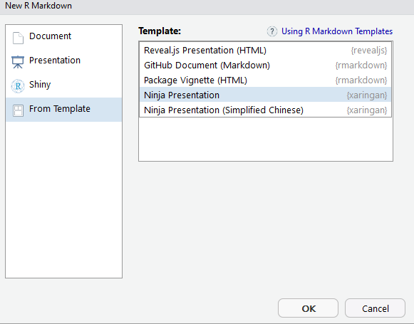
Note: If you understand chinese you can select the last option ;).
The header is going to look like this
---
title: "Presentation Ninja"
subtitle: "⚔<br/>with xaringan"
author: "Yihui Xie"
institute: "RStudio, Inc."
date: "2016/12/12 (updated: 2019-09-23)"
output:
  xaringan::moon_reader:
    lib_dir: libs
    nature:
      highlightStyle: github
      highlightLines: true
      countIncrementalSlides: false
---
A lit bit more complicated than others and as you will see, there are some funny arguments that make this library really different.
css: to add your own CSS file,self_contained: to produce a self-contained HTML fileseal: to generate a title slide automatically using the YAML metadata of the R Markdown document (if FALSE, you should write the title slide by yourself)yolo: to insert the Mustache Karl (TM) randomly in the slides. Using TRUE, a number between 0-1 to insert the Mustache Karl in a percentage of the slides, or even a list(times = n, img = path)chakra: path to the remark.js library (can be either local or remote).nature: (Nature transformation) A list of configurations to be passed to remark.create(), e.g. list(ratio = ‘16:9’, navigation = list(click = TRUE)); see https://github.com/gnab/remark/wiki/Configuration
Besides the options provided by remark.js, there are others such interesting like autoplay the slides or the countdown timer. Slides can be automatically played setting the autoplay option under nature (in milliseconds). For example, to display slides every 30 seconds and see the countdown timer:
---
output:
  xaringan::moon_reader:
    nature:
      autoplay: 30000
      countdown: 30000
---
It is possible to highlight code lines turning the option highlightLines to true or to extend the markdown syntax defining custom macros with the beforeInit option under the option nature.
Adding your CSS file
Some of the previous presentation formats give us the chance to add a customized CSS file. To know how to change a specific element you can inspect it with any web browser and focus exactly on what you want to modify by yourself. An example of a basic modification in a CSS file is the next one. Here we are selecting the background color of the body, the color of the headers and the full text for the reveal presentation, and the size of the h1 header:
body {
  background: #111;
  background-color: #111; }

.reveal {
  color: #fff; }

.reveal h1,
.reveal h2,
.reveal h3,
.reveal h4,
.reveal h5,
.reveal h6 {
  color: #fff;
 }

.reveal h1 {
  font-size: 4.77em; }
Then you have to save the CSS file in the same path that your R presentation document.
How to export the presentation
With all the HTML output it is possible to export the presentation to pdf with any web browser using the menu Print to PDF from Google Chrome, for example. But there is another alternative like publishing the presentation online in RPubs or GitHub. You must be registered in any of the two platforms to be able to add your work. For RPubs, you have to invoke the More -> Publish to RPubs command from the presentation toolbar, and in GitHub, you have to create a new repository with the HTML document and all the style files associated, and enable to GitHub pages to this repository. Here you have the steps to do it: https://pages.github.com/.
Basic example
Finally, let’s show you a simple reveal.js example to get you started.
---
title: "Revealjs Presentation Example"
author: "Paula LC"
date: "September 24, 2019"
output:
  revealjs::revealjs_presentation:
    theme: black
    highlight: pygments
---

## Basic slide with text and lists

Hello world!

- List item 1
- List item 2
  + List item 2.1

## Equations

This summation expression $\sum_{i=1}^n X_i$ appears inline.

$$f(y|N,p) = {{N}\choose{y}} \cdot p^y \cdot (1-p)^{N-y}$$

## Tables

```{r cars, echo = TRUE, results='asis'}
mod <- lm(dist~speed, data=cars)
pander::pander(mod, type = 'html', title = 'Table with pander')
```

## Interactive plot

```{r, echo=FALSE, warning=FALSE}
library(leaflet)

m <- leaflet() %>%
  addTiles() %>%
  addMarkers(lat=40.3325364, lng=-3.7675058, popup="Coding Club UC3M")
m
```

## A background page {data-background-iframe='https://codingclubuc3m.rbind.io'}
After knitting this, here is the result:
Conclusions
RStudio is an awesome framework that provides you the chance to create nice presentations with a simple syntax, adding interactive content, and with a professional and modern style. Moreover, your presentation will be reproducible if you want to make any change, as well as you can save your templates to use them in the future. In my opinion, it is a really good alternative to other traditional software to create presentations and so easy to work with it. I hope it is so useful for you too :)